Multi-Scale and/or Multi-Frequency deconvolution
ASKAPSoft provides a somewhat bewildering array of deconvolution options. This guide aims to point you at the path through these that has proven to give good results.
Spectral line - spectral line cubes have a single frequency per image plane, so you only need decide if you want to use Multi-Scale deconvolution or not
Continuum - for wide band continuum imaging you may need both Multi-Scale deconvolution and Multi-Frequency Synthesis
Here is a list of the current CLEAN deconvolution options:
Hogbom - the classic CLEAN algorithm, deconvolves the sky into delta function components. Implemented using casacore’s LatticeCleaner.
MultiScale - the Multi-Scale CLEAN algorithm, deconvolves the sky into delta functions and tapered parabolas of different sizes. It also uses the casacore LatticeCleaner. Not all the parameters are accessible through the ASKAPsoft interface
BasisFunction - the ASKAPSoft version of multi-scale CLEAN - this version appears to have some flaws when used with scales. Avoid for now.
MultiScaleMFS - Multi-scale Multi Frequency Synthesis, handles multiple scales and decomposes spectral variation with one or more Taylor terms. It uses the casacore MultiTermLatticeCleaner.
BasisfunctionMFS - the ASKAPSoft version of MSMFS, it seems to work slightly better (fewer iterations) but is otherwise very similar.
For most cases we recommend using BasisFunctionMFS with a few scales but Hogbom is often sufficient for a first look at a field. Because the Basisfunction algorithm is not working optimally, use BasisfunctionMFS with nterms=1 (the default) for narrow band work like spectral line cubes.
Choice of Scales
With multi-scale clean you need to choose a set of scales. Usual starting choices are [0,10,30] or [0,4,8,16,32]. The conventional wisdom is that the smallest scale after 0 should be 1-2 times the beam size in pixels. In principle the largest scale is set by the size of the largest extended source in the field. If you are imaging in the galactic plane, this may be as large as half of the image size. However since the maximum size scale you can image reliably is determined by the shortest baseline, you should make sure there is sufficient sensitivity on short baselines to image the largest scale specified or the clean may diverge. In simulations the images come out slightly better with the powers of two scales than with the sparser [0,3,10,30,…] scheme, but using more scales uses more memory and often time as well, so you may need to compromise.
Choice of Number of Taylor terms
For most ASKAP continuum observations (with up to 300 MHz bandwidth) the relative bandwidth is between 20 and 30%. In Taylor term imaging the error in the higher order terms scales with the inverse of the relative bandwidth to the power of the number of terms (df/f)^(-n), so errors go up rapidly for higher orders. The suggested approach is to use nterms=1 or 2 and only go to 3 if there are defects in the image around strong sources that don’t look like calibration errors. Since the errors depend on the signal to noise, it would make sense to use more terms for the stronger sources and fewer for those close to the noise, but at present this is not implemented. Some typical numbers for ASKAP:
Error in spectral index, alpha: 0.25 at 100 sigma, 0.50 at 30 sigma, 1 at 10 sigma.
Error in curvature, beta: ~1 at 100 sigma, quickly rising to ~5 at 30 sigma.
BasisfunctionMFS Options
The BasisfunctionMFS algorithm supports a few options we’ll briefly discuss:
use orthogonal spatial basis functions
use coupled or decoupled residuals
choice of minor cycle peak finding algorithms (MAXBASE,MAXTERM0,MAXCHISQ)
deep cleaning mode, where new components can only be found on top of existing ones
size of the beam/PSF to use for cleaning, the psf width
The first option orthogonalises the basisfunctions in an attempt to reduce crosstalk between the different scales during deconvolution. Tests have not shown great benefits of this. It tends to use more iterations, take longer and produce structure in the residuals of extended sources. On the other hand, it sometimes recovers extended flux slightly better. To try this option you would use:
Cimager.solver.Clean.orthogonal=True
It is off by default, which is the recommended setting.
The second option either directly uses the value found by the peak finding algorithm as the peak residual for each iteration or finds the value of the maximum across all basisfunction residual images and terms at the peak location. Generally, there is little difference between these but the first value (decoupled) behaves more like in classical clean, i.e., it tends to decrease monotonically as iterations progress whereas the second value can meander up and down a bit (and sometimes gets stuck on a single value for a while) when it is reporting values from a different scale. The default setting is coupled, but we have found that decoupled allows the use of a lower minor iteration percentage limit and is often slightly faster. The deep cleaning mode discussed below always uses decoupled=True. To use decoupled components specify:
Cimager.solver.Clean.decoupled=True
The third choice is the peak finding algorithm.
MAXCHISQ, the default, works well for nterms>1 in most cases. It uses a chi-square image for peak finding that tries to minimise the residuals across all Taylor terms.
MAXTERM0, does not seem to be very useful as the clean often fails to converge using this measure. It uses the Taylor term 0 coefficient image to find the next peak.
MAXBASE, searches the highest peak across the different scales in the Taylor 0 images. It works well and is better than MAXCHISQ at low S/N ratios.
At high S/N and nterms>1 the residuals around strong sources look better with MAXCHISQ. With all options you can reduce the (sinc-function like) error patterns around strong sources and increase the dynamic range by reducing the cell size so you have 3 or more pixels per beam. The MAXCHISQ option can be slower for large images due to the extra calculation of a chi-square image. It will also pick up more spurious noise components when cleaning close to the noise level because the noise in the chi-square image is roughly sqrt(nterms) times higher than the residual image noise. We recommend using MAXBASE for nterms=1 (e.g., spectral line imaging) and cleaning below 10 sigma. To use MAXBASE specify:
Cimager.solver.Clean.solutiontype=MAXBASE
The deep cleaning mode (borrowed from wsclean) can be used to clean below the noise level. Normally you can clean a large area to about 4-5 sigma, without getting too many spurious noise components. The deep cleaning mode uses the existing components as a mask to clean deeper. This can be effective for extended sources that need to be cleaned to <1 sigma to reduce the sidelobes and fully capture all the flux. In Miriad or CASA you would set clean boxes around these sources or use automatic clean boxes, but using the existing model as a mask seems to work quite well too. To use the deep clean feature specify a second absolute flux threshold and lower the major cycle threshold as well:
Cimager.threshold.minorcycle=[40%,2mJy,0.18mJy]
Cimager.threshold.majorcycle=0.2mJy.
Here set the second minor cycle threshold slightly lower than the major cycle threshold to avoid doing several major cycles close to the final level at the end due to small errors.
Another parameter that is worth mentioning is psfwidth. This specifies the size of the psf (dirty beam) used in minor cycle (image based) cleaning. It can affect the run time of your clean a lot. If you have a rather poor beam with large sidelobes setting this large can help to avoid your clean diverging. If you leave it unset, the full beam is used. The sparser uv coverage of spectral line observations means that you may need to use a large psf width. Continuum imaging using MFS gives much better uv coverage and a smoother beam allowing you to set this much smaller, e.g., 256 or 512. This can speed up your clean minor cycles by a large factor. Because the major cycle subtractions can be parallelised over many cores, but the minor cycle is still running on a single core, a lot of core time is wasted if the minor cycles are slow. As the ASKAP array grows in size and we need to make bigger, higher resolution images, we should hopefully be able to decrease this parameter to speed up the minor cycles. Note that speed gains are limited below 256. Specify the psf width using:
Cimager.solver.Clean.psfwidth = 256
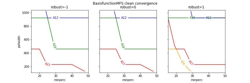
Here is a handy summary plot of the areas in psfwidth and minor cycle percentage limit where clean convergence tends to be good for different sizes of ASKAP. Stay above and to the right of the relevant line in the plot. For ASKAP36 and robust=-1 or 0 the clean converged well for all tested values.
Example 1: Spectral line cubes
For spectral line imaging use the following selection of options:
BasisfunctionMFS solver
standard basisfunctions,
decoupled residuals,
MAXBASE peak finding algorithm,
deep cleaning,
larger psf width
Here is an example parset file that uses multiscale deconvolution and deep cleaning, replace <object> with the appropriate value for you:
Cimager.dataset         = <object>.beam00_SL.ms
Cimager.imagetype       = casa
#
Cimager.Images.Names    = image.i.<object>.cube.b00
Cimager.Images.shape    = [1536, 1536]
Cimager.Images.cellsize = [4arcsec, 4arcsec]
# Replace direction as needed
Cimager.Images.direction= [13h37m54.000, -29.43.49.62, J2000]
Cimager.Images.restFrequency = HI
# Options for the alternate imager
Cimager.nchanpercore    = 54
Cimager.usetmpfs        = false
Cimager.tmpfs           = /dev/shm
# barycentre and multiple solver mode not supported in continuum imaging (yet)
Cimager.barycentre      = true
Cimager.solverpercore   = true
Cimager.nwriters        = 1
Cimager.singleoutputfile= false
#
# This defines the parameters for the gridding.
Cimager.gridder.snapshotimaging             = true
Cimager.gridder.snapshotimaging.wtolerance  = 2600
Cimager.gridder.snapshotimaging.longtrack   = true
Cimager.gridder.snapshotimaging.clipping    = 0.01
Cimager.gridder                             = WProject
Cimager.gridder.WProject.wmax               = 2600
Cimager.gridder.WProject.nwplanes           = 99
Cimager.gridder.WProject.oversample         = 4
Cimager.gridder.WProject.maxsupport         = 512
Cimager.gridder.WProject.variablesupport    = true
Cimager.gridder.WProject.offsetsupport      = true
#
# These parameters define the clean algorithm
Cimager.solver                              = Clean
Cimager.solver.Clean.algorithm              = BasisfunctionMFS
Cimager.solver.Clean.niter                  = 5000
Cimager.solver.Clean.gain                   = 0.1
Cimager.solver.Clean.scales                 = [0,3,10,30]
Cimager.solver.Clean.verbose                = False
Cimager.solver.Clean.tolerance              = 0.01
Cimager.solver.Clean.weightcutoff           = zero
Cimager.solver.Clean.weightcutoff.clean     = false
Cimager.solver.Clean.psfwidth               = 512
Cimager.solver.Clean.logevery               = 50
Cimager.solver.Clean.solutiontype           = MAXBASE
Cimager.solver.Clean.decoupled              = True
Cimager.threshold.minorcycle                = [40%, 9mJy, 1mJy]
Cimager.threshold.majorcycle                = 1.1mJy
Cimager.ncycles                             = 10
Cimager.Images.writeAtMajorCycle            = false
#
Cimager.preconditioner.Names                = [Wiener]
Cimager.preconditioner.preservecf           = true
Cimager.preconditioner.Wiener.robustness    = 0.5
#
# These parameter govern the restoring of the image and the recording of the beam
Cimager.restore                             = true
Cimager.restore.beam                        = fit
Cimager.restore.beam.cutoff                 = 0.5
Cimager.restore.beamReference               = mid
Example 2: Continuum Imaging
In continuum imaging you tend to be limited by calibration errors instead of noise, so make sure you keep the first absolute clean level above the level of the calibration errors. You can still use deep cleaning to collect all the flux of sources above that level (e.g., for selfcal purposes). Here the suggested options for continuum imaging:
BasisfunctionMFS solver
standard basisfunctions,
2 Taylor terms
decoupled residuals,
MAXCHISQ or MAXBASE peak finding algorithm,
deep cleaning,
choose a smaller psf width
Here is an example parset for continuum imaging:
## Continuum imaging with cimager
##
#Standard Parameter set for Cimager
Cimager.dataset                                 = <object>.beam00_averaged.ms
Cimager.datacolumn                              = DATA
Cimager.imagetype                               = casa
#
# Each worker will read a single channel selection
Cimager.Channels                                = [1, %w]
#
Cimager.Images.Names                            = [image.<object>.beam00]
Cimager.Images.shape                            = [3200, 3200]
Cimager.Images.cellsize                         = [4arcsec, 4arcsec]
# Enter the correct direction for your observation
Cimager.Images.<object>.beam00.direction        = [13h37m54.000, -29.43.49.62, J2000]
# This is how many channels to write to the image - just a single one for continuum
Cimager.Images.<object>.beam00.nchan            = 1
#
# The following are needed for MFS clean
# This one defines the number of Taylor terms
Cimager.Images.<object>.beam00.nterms           = 2
# This one assigns one worker for each of the Taylor terms
Cimager.nworkergroups                           = 3
# Leave 'Cimager.visweights' to be determined by Cimager, based on nterms
# Leave 'Cimager.visweights.MFS.reffreq' to be determined by Cimager
#
# Options for the alternate imager
Cimager.nchanpercore                           = 1
Cimager.usetmpfs                               = false
Cimager.tmpfs                                   = /dev/shm
# barycentre and multiple solver mode not supported in continuum imaging (yet)
Cimager.barycentre                              = false
Cimager.solverpercore                           = false
Cimager.nwriters                                = 1
#
# This defines the parameters for the gridding.
Cimager.gridder.snapshotimaging                 = true
Cimager.gridder.snapshotimaging.wtolerance      = 2600
Cimager.gridder.snapshotimaging.longtrack       = true
Cimager.gridder.snapshotimaging.clipping        = 0.01
Cimager.gridder                                 = WProject
Cimager.gridder.WProject.wmax                   = 40000
Cimager.gridder.WProject.nwplanes               = 99
Cimager.gridder.WProject.oversample             = 5
Cimager.gridder.WProject.maxsupport             = 1024
Cimager.gridder.WProject.variablesupport        = true
Cimager.gridder.WProject.offsetsupport          = true
#
# These parameters define the clean algorithm
Cimager.solver                                  = Clean
Cimager.solver.Clean.algorithm                  = BasisfunctionMFS
Cimager.solver.Clean.niter                      = 4000
Cimager.solver.Clean.gain                       = 0.1
Cimager.solver.Clean.scales                     = [0,4,8,16,32]
Cimager.solver.Clean.verbose                    = False
Cimager.solver.Clean.tolerance                  = 0.01
Cimager.solver.Clean.weightcutoff               = zero
Cimager.solver.Clean.weightcutoff.clean         = false
Cimager.solver.Clean.solutiontype               = MAXBASE
Cimager.solver.Clean.decoupled                  = True
Cimager.solver.Clean.psfwidth                   = 256
Cimager.solver.Clean.logevery                   = 50
Cimager.Images.writeAtMajorCycle                = false
Cimager.threshold.minorcycle                    = [30%,0.5mJy,0.1mJy]

#
Cimager.preconditioner.Names                    = [Wiener]
Cimager.preconditioner.preservecf               = true
Cimager.preconditioner.Wiener.robustness        = -0.5
#
Cimager.restore                                 = true
Cimager.restore.beam                            = fit
Cimager.restore.beam.cutoff                     = 0.5

#
Cimager.threshold.majorcycle                    = 0.11mJy
Cimager.ncycles                                 = 10
# Excluding the shortest baselines can avoid large scale ripples due to RFI
Cimager.MinUV   = 30