Reduction Strategies

Here we give an overview of the reduction process, and review some of the basic decisions that you will have to make during the reduction of the data. We now consider some questions that you should ask yourself before the reduction process.

• Is this observation more than a single-pointing, continuum experiment? Hopefully the answer to this is obvious! This manual contains special chapters addressing the reduction of spectral line (Chapter 16), mosaic (Chapter 21) and pulsar-bin mode (Chapter 24) observations. You are encouraged to review appropriate chapters before you start reducing your data.

• Will I want to deconvolve my images? Deconvolution is the process of removing artifacts due to the incomplete sampling in the u-v plane. You will want to deconvolve for observations where the source is stronger than a few times the noise limit. That is, unless you are doing a detection experiment, you are likely to want to deconvolve. Deconvolution is addressed in Chapter 14.

• Will I want to self-calibrate the data? Self-calibration is the process of determining the antenna-based gain function from the source itself. For this to be possible, your signal needs to be about 5 to 10 times stronger than the thermal noise when integrated over the self-calibration solution interval (typically 15 seconds to 5 minutes). For the ATCA in continuum mode, this means a source which contains at least 100 to 200 mJy in most baselines. Self-calibration is discussed in Chapter 15.

• As I have a continuum experiment, do I want to use multi-frequency techniques? Even in continuum mode, the ATCA produces multiple channels of data. As the fractional bandwidth can be quite significant, you may be making a significant approximation if you average all these channels into a single channel (the so-called `channel-0' dataset). The result will be poorer u-v coverage and bandwidth smearing. If you are interested in high dynamic range imaging, or if a good beam is important, and you are observing at 21, 13 and possibly 6 cm, then it is best not to average your data into a single channel. Rather you can calibrate and form a single image directly using the multichannel data. This practise is known as multi-frequency synthesis.

  Multi-frequency synthesis can be taken a few steps further with the ATCA. As two IFs can be measured simultaneously, these two IFs can be combined in the imaging stage to further enhance both sensitivity and u-v coverage. As the ATCA can frequency switch rapidly, it is possible to time share between different frequency settings. This involves a trade-off between tangential and radial u-v gaps.

• Should I average my data in time or frequency? The reason to average your data is to reduce you disk consumption and to increase the speed of the various processing programs. If these practical considerations are important, you may consider averaging your data in time and frequency. In this case, you probably want to do this as early as possible in the reduction process - after the initial flagging.

  Frequency averaging is generally only applicable for continuum experiments and only if you are not going to be doing multi-frequency synthesis. You might also think twice about averaging if interference was a problem during the observation. You may have to go back and do some more flagging later.

  Averaging in time can be performed when observing with short arrays (i.e. when the 6 km antenna is not used). A conservative rule is that you should not average longer than 90/d seconds, where d is the array length in km. If you observe with a short array and are not interested in long baselines for the program source, you probably still want to use antenna 6 when determining the initial calibration. Despite this, d is the array length of interest for the program source, not the calibrators. Nor should you average for longer than the antenna-gain solution interval (unless you have finished calibrating, and are not going to self-calibrate). If you have a strong source, and the phase stability is poor, you should not average in time.

  Both averaging in frequency and time are performed by uvaver (see Section 10.4).

Figure 7.1: ATCA Data Reduction Strategy

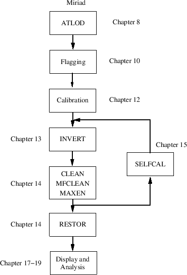
Figure 7.1 gives a flow chart of the normal steps involved in reduction of ATCA data. Note that this is somewhat abbreviated by necessity - additional flow-charts in subsequent chapters give more detail and describe some of the variations.

We will now consider each step in the flow-chart in turn.

1. Data from the ATCA is written in ``RPFITS'' format - an ATNF-specific format - and a special task (atlod) is needed to read it. Loading your data into Miriad is described in Chapter 8.

2. Data editing (flagging) can be very time consuming, especially if you do are affected by interference. The Miriad flagging tasks are described in Chapter 10.

3. The actual calibration steps can be the most confusing steps, as there are a large variety of paths that can be followed. Only the most frequently trodden paths are described in Chapter 12.

4. The task invert takes a visibility dataset and forms either a single image or an image cube (for spectral-line observations). It also produces a point-spread function (dirty beam), ready for deconvolution. See Chapter 13

5. The main deconvolution tasks are clean, maxen and mfclean. Task clean, which is the most commonly used, attempts to decompose your image into a number of delta functions. It can be slow for images with a large amount of extended emission. An alternative to clean is maxen, a maximum entropy-based deconvolution task. It tends to be less robust and more difficult to run correctly. A third alternative is mfclean. This is a derivative of the CLEAN algorithm, and simultaneously determines a flux density and spectral index image. It is only appropriate for multi-frequency synthesis experiments when more than one observing band has been used.

   The deconvolution tasks are described in Chapter 14.

6. As noted above, self-calibration is useful for determining antenna gains directly from a strong program source. It is described in Chapter 15.
7. The deconvolution tasks produce an output image that is in units of flux density per pixel. That is, the outputs are CLEAN component images. Task restor converts these to flux density per CLEAN beam, and adds back the residuals. This is covered in Chapter 14.
8. At last, you are ready to display and think about your images!