Millimetre-wave spectral line observing with Mopra
The history of the Mopra telescope and my inordinately long PhD are intertwined. In the past seven years Mopra has grown into a fine young telescope. Meanwhile, my PhD, after a long and difficult confinement, has become a description of the capabilities and potential of the Mopra telescope. I would now like to share what I have learned with other potential users.
My PhD has involved observing a large sample of dense cores in southern molecular clouds, in a variety of molecular transitions at millimetre wavelengths. I have used the observed line intensities to calculate molecular abundances and physical conditions in the sample of dense cores. This type of analysis requires careful intensity calibration of the Mopra observations. Consequently, calibration has formed a major part of my thesis.
Intensity Calibration of Mopra Data: Removing the Earth's atmosphere.
The specifics of intensity calibration can be found on the Mopra website at http://wwwnar.atnf.csiro.au/mopra/calibration/mm_calibration.html or http://newt.phys.unsw.edu.au/~ramesh/. Alternatively, I am very happy to send information about Mopra calibration on request to mhunt@atnf.csiro.au. In this article I would like to concentrate on the efficacy of the intensity calibration.
There seems to be a general belief that a millimetre site must be high enough to induce altitude sickness in the unfortunate observer if accurate line intensities are to be obtained. This is not true in the 3-mm band at which Mopra operates. The Earth's atmosphere absorbs radiation at millimetre wavelengths and this effect must be calibrated out, however it has proved possible at Mopra to formulate a calibration method that does this quite effectively. This method is a variation on the "chopper wheel" method commonly used to calibrate millimetre-wave telescopes (see Mopra web site for more information).
The calibration of Mopra data is a two step process:
1) The effect of atmospheric attenuation must be removed from the data. This is a most important step as atmospheric attenuation varies with air temperature, moisture content and zenith angle;
2) Secondly, the data must be tied to a known brightness temperature (intensity) scale. In this case the Mopra observations have been placed onto the SEST antenna temperature scale.
How effectively can this be done?
Figure 1 compares SEST observations to Mopra observations for the chosen primary calibrators Orion A and M 17. Figure 1a shows the Mopra observations before atmospheric calibration (QT) and Figure 1b shows the Mopra observations after atmospheric calibration (TA'). The Mopra observations were made at a range of frequencies between 86 and 115 GHz during the period 1995 to 1998, in weather conditions that varied from clear to heavy cloud cover. The SEST observations are available on the SEST web site at http://www.ls.eso.org/lasilla/Telescopes/SEST/SEST.html.
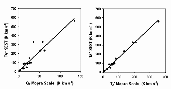
Figure 1: Comparison of SEST and Mopra data before and after calibration of the Mopra data. (a) SEST corrected antenna temperature (TA*) plotted with Mopra peak antenna temperature before calibration (QT). The equation for the line of best fit is (TA* SEST = 4.33(QT MOPRA) + 7.3 and the correlation coefficient is r2 = 0.87. (b) SEST corrected antenna temperature (TA*) plotted with corrected peak antenna temperature from Mopra (TA') for the same data after calibration. The equation for the line of best fit is (TA* SEST = 1.62(TA' MOPRA) _ 1.1 and the correlation coefficient is r2 = 0.99.
The atmospheric calibration method clearly removes the attenuation effectively. The calibrated Mopra observations can then be placed on the SEST antenna temperature scale using the linear fit from Figure 1b. This relationship is
TA*(SEST) = (1.62 ± 0.06)TA'(Mopra). (1)
Note that this relationship is only valid for data collected prior to the resurfacing of the Mopra dish in 1999.
The correlation coefficient for equation (1) is r2 = 0.99.
Uncertainties in Mopra Data
The uncertainties in the Mopra data themselves have been calculated from repeated observations of a set of secondary calibrators. Once again the Mopra observations were collected during the period 1995 _ 1998 in a variety of weather conditions.
The relative difference of each observation from the mean for that source (in terms of integrated brightness temperature), at that frequency, is shown in Figure 2. The observations are plotted against integrated main-beam brightness temperature (TMBDv) from calibrated Mopra observations. The uncertainties have been modelled as consisting of a flux dependent and a flux independent component as described in equation 2.
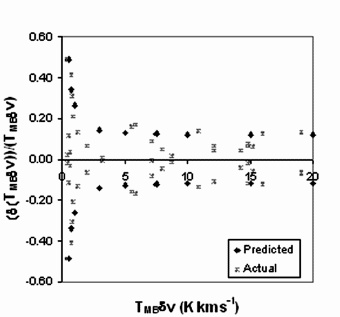
Figure 2: Relative uncertainties computed from equation (2) compared with actual values of relative uncertainties for calibrated Mopra data, plotted with integrated main-beam brightness temperature. The diamonds show the predicted values, while the crosses show the values obtained from repeated measurements.
The sum of the two uncertainties can be represented by
![]() (2)
(2)
where TMB is the calibrated Mopra main-beam brightness temperature.
Figure 2 also shows the uncertainty values predicted by equation (2).
Calculating the uncertainties in this empirical way takes into account all sources of error, including those from the Gaussian fit to the spectral line. The flux-independent uncertainty of 11.8 per cent compares well with that of the SEST, which is estimated to be 10 per cent at 3-mm.
Doing Science with Mopra
Of course the proof of the pudding is in the eating. The rotation diagram in Figure 3 shows that Mopra can be used just as well as SEST to do science with 3-mm observations.
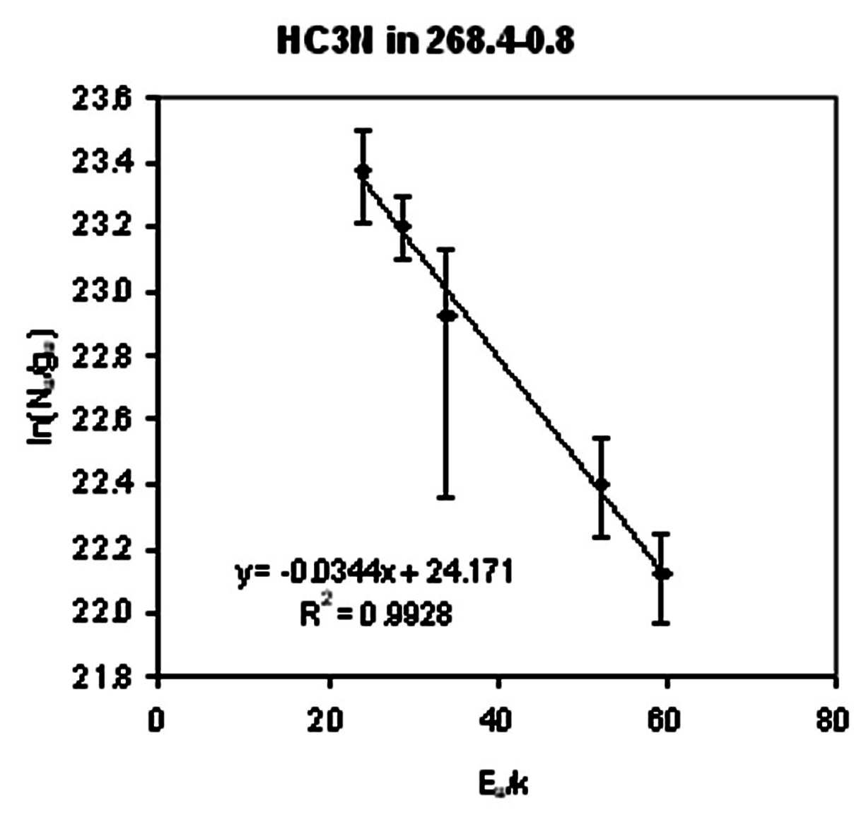
Figure 3: Rotation diagram for HC3N in G268.4-0.8.
The rotation diagram (Figure 3) shows the number of molecules per statistical weight in the upper level of a transition plotted with the energy of the level above the ground state. The transitions shown, in order of increasing energy, are J=10-9, J=11-10, J=12-11, J=15-14 and J=16-15. The J=10-9 and J=12-11 are from Mopra whereas the others are from the SEST. The straight line relationship shows that the MOPRA and SEST observations have been successfully calibrated onto the same scale, as well as giving information about the excitation in the G268.4-0.8 molecular cloud.
The capacity of Mopra to provide accurate measurements of molecular line intensities makes it a valuable tool for investigating the interstellar medium and evolved stars, either used on its own or in conjunction with the SEST. The ready availability of Mopra to Australian astronomers and the low associated travel costs add to its value.
Studying the Interstellar Medium
Accurate measurements of molecular line intensities in several transitions of a molecule can be used to determine molecular abundances, temperatures and densities within molecular gas. There are a number of ways to obtain this information, all starting of course with the crucial business of accurate well-calibrated observations.
The kinetic temperature and molecular hydrogen column density can be obtained from observing CO and its isotopomers 13CO, C18O and C17O. The methods for doing this can be found in Rohlfs and Wilson (1996). The kinetic temperature is the temperature of the molecular hydrogen in a dense molecular cloud. CO can be assumed to be thermalised at the kinetic temperature. Other molecules may have different excitation temperatures, depending on the relative importance of their interaction with both the hydrogen molecules and the radiation field within the molecular cloud. (The radiation field at any frequency will have its own characteristic temperature as defined by Planck's law.)
A rotation diagram can be used to find the molecular abundance and excitation temperature of a molecule, if a straight line fit can be obtained. This type of local thermodynamic equilibrium (LTE) analysis can be used if the emission in the observed transitions is optically thin and if all transitions have the same excitation temperature (as defined by the level populations and the Maxwell-Boltzmann equation). For molecules such as HCN, HCO+ and CS, which are usually optically thick, observations of 13CO isotopomers can be used for the rotation diagram. A good reference for the use of the rotation diagram as an analytical tool can be found in Goldsmith and Langer (1999).
If the conditions of low optical depth and a single excitation temperature for all transitions are not met, a large velocity gradient (LVG) analysis can be used although this is a considerably more complex undertaking. An LVG analysis can give the kinetic temperature, excitation temperature, hydrogen spatial density and molecular abundance if at least four different transitions have been observed. I have some LVG analysis programs that I would be happy to provide to interested parties.
Combining Mopra with the SEST
The molecules HC3N and OCS have three transitions within the range of Mopra, and CH3OH has six. Mopra observations alone can be sufficient to determine physical conditions in these sources if combined with information on the kinetic temperature and molecular hydrogen column density from observations of CO. Molecular abundances can also be estimated from observations of a single molecule if the conditions for an LTE analysis are met. The optical depth is determined by observing an optically thin isotopomer of the molecule in question; however, observing a single transition does not give information on the excitation temperature of the molecule and so the accuracy of the abundance estimate cannot be known without further information.
The best strategy is to use Mopra to observe the available transitions of the molecules of interest and then augment these observations with SEST observations of some 2-mm and 1-mm transitions of the same molecule.
References
Goldsmith and Langer, 1999. ApJ. 517, 209.
Rohlfs, K., and Wilson, T. L. 1996, Tools of Radio Astronomy, 2nd Edition. p. 386. Springer-Verlag, Berlin.
Maria Hunt, University of Western Sydney
(mhunt@atnf.csiro.au)