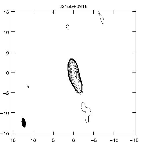
Figure 1: Total intensity plot of the scintillating extragalactic radio source J2155+0916. Thin contours are in steps of 2 with the lowest contour at 0.3-sigma. The single thick "fiducial" contour indicates 2 % of the peak flux.
As part of a project to investigate milli-arcsecond scale morphological differences between scintillating and non-scintillating flat spectrum radio sources we needed to do something that seemed fairly simple: display the same image using, simultaneously, two different kinds of contours. This was needed to indicate the location of a "fiducial" contour that was defined as a fraction of the peak flux and was to be used as an indication of how extended a source is. The sources in this sample have very weak extended structure for which the traditional model fitting method (typically using the Modelfit program from the Caltech Difmap package) does not yield objective results.
To our surprise, we were unable to find a way to
do this using the traditional astronomy packages we
were familiar with. We discovered, however, that it
is possible to do this using aips++. Malte
Marquarding and Neil Killeen of the aips++ group
immediately wrote a script to produce an image which
could display two different kinds of contours where
the contours can be distinguished in various ways such
as width and colour.
Figure 1: Total intensity plot of the
scintillating extragalactic radio source J2155+0916. Thin
contours are in steps of 2 with the lowest contour at
0.3-sigma. The single thick "fiducial"
contour indicates 2 % of the peak flux.
Having achieved our basic requirement Malte has greatly expanded the original script to one that generates all our total intensity, polarization and fractional polarization plots for this project. This script is designed for batch processing large numbers of sources while still providing interactive modification for individual sources. This does at least everything that AIPS can and does so with greater flexibility and, arguably, ease of use. The high level of prompt support from the ATNF aips++ group has eased our transition to the use of aips++.
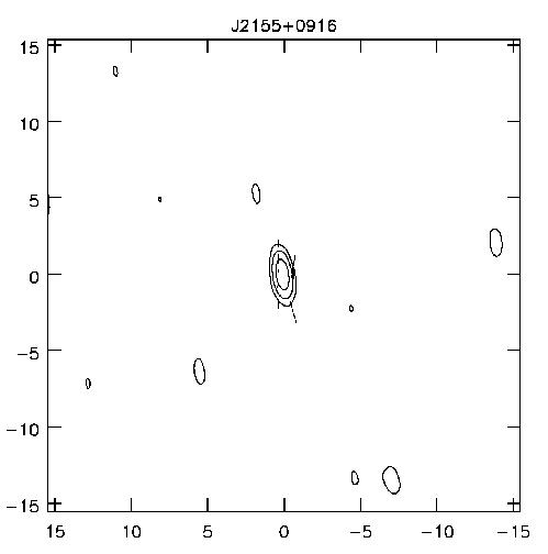
Figure 2: Polarized intensity contours for
J2155+0916. Contours are in steps of 2 with the lowest contour
at 3-sigma. The tick marks indicate the direction of
the electric vector position angle. Their spacing
and length have no significance.
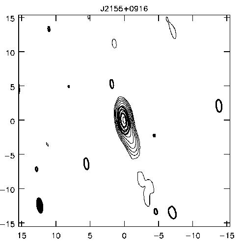
Figure 3: Fractional polarization plot for J2155+0916. The thin contours show total
intensity exactly as in Figure 1. The thick contours
show the polarized intensity as in Figure 2.
Roopesh Ojha
(Roopesh.Ojha@csiro.au)