Demonstration of widefield continuum and polarisation capabilities on Mk I PAFs
|
|
3 December 2014
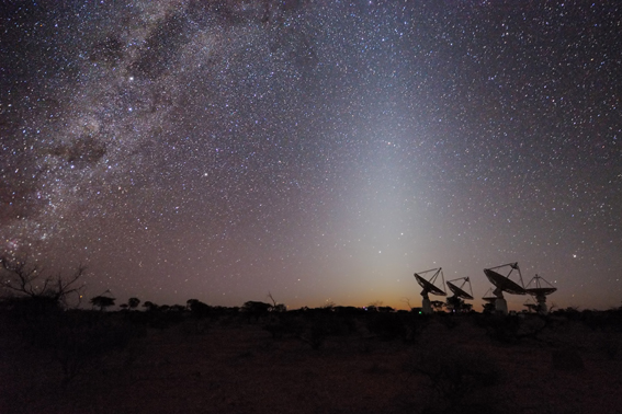
Widefield continuum imaging has been successfully demonstrated on BETA using Mk I PAFs. As proof we make available a full-Stokes image of a region in the southern constellation Tucana, made over the frequency range 700 - 1000 MHz ('BETA band 1').
Below we set out some properties, and caveats, of the image. We also guide the interested user on how to access the data and we give a summary of the procedures followed to produce the image.
Properties:
- Observations were made on 11-09-2014, and 13-09-2014 (scheduling block numbers SBID = 609,617). These observations include brief observations of the southern calibrator B1934-638 (SBIDs 608,616) made with all beams.
- The observations were made with the Square beam footprint with beam pitch of 1.46 degrees. Each observation of the target was made with two antenna pointings, alternated every 1000s. The pointings (J2000 coordinates) were (22:40:00.000,-60:00:00.00) and (22:45:58.305,-60:43:18.55).
- The final image covers an area of approximately 31 square degrees. The image noise over most of that area is approximately 0.45 mJy/beam. The restoring beam for the image has size 76 x 56 arcseconds.
- Images of the area have been made for Stokes quantities I, Q, U and V. Be aware that the data are not polarimetrically calibrated. They are produced to demonstrate that all polarisation products are correlated and passed through the system software, but the Q, U and V images should NOT be used for any scientific interpretation.
Caveats:
- A deficiency of BETA is its lack of a noise-injection scheme from which to measure the interferometric phase difference between the X and Y polarisations - the so-called X-Y phase. This means that the Q and V images are unknown linear combinations of the true Q and V.
- B1934-638 was used to calibrate the gain bandpass, but no attempt was made to solve for and correct for polarisation leakages. In separate experiments, these leakages have been measured and are low (~0.5%) and stable over periods of weeks.
- From other polarimetric investigations, we know that the gains of the X and Y beams differ away from the beam centre. No attempt has been made in the observations of Tucana to quantify or correct these differences. This will degrade the polarimetric performance away from beam centres.
- The lack of polarimetric polarisation also means that the total intensity (I) of intrinsically polarised sources will be in error to some degree.
The images are available at the following links:
The raw data are held at the Pawsey Centre on storage attached to computer "galaxy". Data are in the form of MeasurementSet files, readable by both ASKAPsoft and casa.
Interested users are invited to ask CSIRO (by email request to David McConnell, Lisa Harvey-Smith or Aidan Hotan) for an account on the Galaxy supercomputer at the iVEC Pawsey Centre, and read the relevant documentation on accessing ASKAP data.
Steps taken in the data processing:
- Use task cflag (see http://www.atnf.csiro.au/computing/software/askapsoft/sdp/docs/current/c...) for a preliminary flagging on the full resolution data; use an amplitude threshold of about 1.0 (this value may not suit all datasets). Do this on both calibrator and target measurement sets.
- Use task mssplit to split the measurement set into beam-specific files, and at the same time average in frequency to 304 1MHz channels. Do this on both calibrator and target measurement sets.
- Form bandpass calibration tables from scan i of beam i data ( for i in [0..8]) from the calibration (B1934-638) data. Additional flagging may be necessary to get good quality bandpass corrections.
- Apply the bandpass calibration, beam for beam, to the target datasets.
- Split the target datasets into eight spectral bands, each 38 MHz wide. There are now 72 bandpass calibrated sets of visibility data.
- Image and deconvolve each visibility dataset with an image size that encompasses the 2nd side lobe (about 13.5 degrees, full width).
- From each image, construct a model from the sources brighter than ~10 sigma. Use this model for phase-only self cal of the corresponding visibility data, and image again.
- Form the linear mosaic from all beams, using an appropriate primary beam model. The choice of primary beam model is continually being refined as we learn more about the beam shapes.