ASKAP Array Configuration
The text below forms a paper 'The initial array configuration for ASKAP' by Neeraj Gupta, Simon Johnston, Ilana Feain and Tim Cornwell. The PDF can be found here [2.6MB PDF]. Note that the PDF version does not contain any of the revisions added to these web pages.
For all enquiries or further information, please contact the ASKAP Project Scientist.
Revision History
1.0 - 31 October 2008: Live version
1.1 - 1 November 2008: Completed table 3 with surface brightness sensitivities for 10 and 18 arcsec resolution
1.2 - 5 November 2008: Made clear in tables 2 and 3 that sensitivities are 1-sigma
1.3 - 5 November 2008: The effects of confusing sources are not considered in Tables 2 and 3. Consult the Condon memo for more information.
1.4 - 14 November 2008: Added in beam size for +30 and +40 declination into Table 1
1.5 - 14 November 2008: Added in hour angle coverage versus declination as Figure 5
1.6 - 11 December 2010: Added information about the antenna positions
1.7 - 28 February 2013: Updated the current set of antenna positions
Antenna Locations (updated 28 February 2013)
The current surveyed measurements of the locations of the ASKAP antennas can be found in this spreadsheet. These locations are the surveyed locations of the centres of the pedestal bases. Locations of the centre of the receivers are not yet available for most antennas. These locations differ from the locations contained in the document below which was an ideal configuration (but which did take into account the site mask). The differences are small and are mostly due to the nature of terrain.
The surveyed measurements are the Easting and Northing values for each antenna. From these, the values of the longitude and latitude have been derived, which are included in the spreadsheet. This was done with the MGA Transverse Mercator projection, using MGA zone number 50.
The BETA antennas are numbers 1, 3, 6, 8, 9 and 15 – as indicated in the spreadsheet. Also included are the antenna names, as provided by the local Wajarri Yamatji community.
KML fils for the full ASKAP array and for the BETA antennas only are available; these can be used in Google Earth and also on Google Maps.
Initial Array Configuration Overview
The science cases for ASKAP (Johnston et al. 2007, Johnston et al.2008) were written without specific configuration details. Subsequently, science priorities for ATNF telescopes in general and ASKAP in particular were presented in ATNF Science in 2010-2015 (pdf file) by Ball et al. (2008), and this priority listing strongly influenced the configuration decision.
Input from the community at large and the ASKAP Science Working Group were also taken into consideration. An initial discussion paper for ASKAP configurations was given by Feain et al.(2008) with the technical studies presented in ASKAP Array Configurations: Technical Studies, Gupta et al. (2008). We recommended that the best initial option for the configuration was a hybrid array optimised for the HI emission surveys.
The overall ASKAP budget envelope has since established that the initial configuration will consist of 36 antennas. The configuration derived in this paper has 30 of the antennas arranged within a circle of diameter 2 km, with a further 6 antennas arranged to form a Reuleaux triangle with maximum separation of 6 km. The configuration takes into account a mask of the site at the Murchison Radio-astronomy Observatory (MRO).
The initial ASKAP configuration is optimised to produce excellent sensitivity and a good point spread function (sidelobe levels 2-3%) at an angular resolution of 30'' at 1.4 GHz. The configuration also provides high survey speed at an angular resolution of 10'' and good surface brightness sensitivity at angular resolutions of 60'' and 90''. We expect that this configuration will return excellent science outcomes for ASKAP for at least the first five years of its operation.
Introduction
ASKAP is a next generation radio telescope on the strategic pathway towards the staged development of the SKA. ASKAP has four goals:
- to demonstrate and prototype the technologies for the mid-frequency SKA, including field-of-view enhancement by focal-plane phased arrays on new-technology 12-metre class parabolic reflectors,
- to carry out world-class, groundbreaking observations directly relevant to the SKA Key Science Projects,
- to establish a site for radio astronomy in Western Australia where observations can be carried out free from the harmful effects of radio interference,
- to establish a user community for SKA.
ASKAP will become operational from 2012, SKA Phase I will become operational from 2015, and full SKA will become operational from 2020. The default lifetime of ASKAP is 30 years and current planning assumes this default. However, the practical lifetime of ASKAP is likely to be much shorter if the Murchison Radio-astronomy Observatory is chosen as the site for the SKA - this decision will be made in 2011-12. Regardless of where the SKA is built, it is crucial that ASKAP return the best science outcomes during its first 5-7 years of operation; this is ASKAP's competitive lifetime. Beyond this time ASKAP will be superseded by SKA phase I, and eventually SKA.
A summary of the science case for ASKAP was presented in Johnston et al. 2007 with a more complete version in Johnston et al. (2008, in press). The science case was written before the exact number of antennas was known and without a specific configuration; the only constraint was that the maximum baselines be less than 8 km.
The science priorities for ASKAP in the period 2010-2015 are presented as part of the Ball et al. (2008) document ATNF Science Priorities in 2010-2015. As listed in that document, the order of science priorities for ASKAP is:
- Understanding galaxy formation and gas evolution in the nearby Universe through extragalactic HI surveys, including near-field cosmology
- The characterisation of the radio transient sky through detection and monitoring (including VLBI) of transient and variable sources
- Determining the evolution, formation and population of galaxies across cosmic time via high resolution, confusion-limited, continuum surveys
- Exploring the evolution of magnetic fields in galaxies over cosmic time through polarisation surveys
Since the time of writing of those documents, the number of antennas available to ASKAP has been finalised to be 36. In this document we present the initial ASKAP configuration, show the UV coverage and beam shapes for various declinations and describe the sensitivity as a function of angular resolution.
Configuration
The science priorities, in conjunction with the recommendations in Feain et al. (2008), the studies by Gupta et al. (2008) and community consultation have resulted in the initial configuration of ASKAP which seeks to maximise the sensitivity for extragalactic HI surveys (Staveley-Smith 2006, 2008) whilst also providing high resolution and good surface brightness sensitivities.
To achieve this, the locations of 27 antennas were optimised using AntConfig (de Villiers 2007) to produce a Gaussian distribution of visibilities with a scale of ~700m, corresponding to a point spread function of ~30". Three antennas were then added to the core of the configuration to provide short spacings (20-100 m) to enhance the low surface brightness sensitivity. Finally, six antennas were arranged to form a Reuleaux triangle with a maximum separation of 6 km.
The layout of the 36 antennas is shown in Figure 1. The configuration has a smallest antenna separation of 22 m, and a longest separation of 6 km.

Figure 1: Layout of the 36 antennas of the initial ASKAP configuration. The circle has a radius of 1 km.
ASKAP is located on the Murchison Radio-astronomy Observatory in the Murchison Shire of Western Australia. The longitude and latitude, corresponding to the 0,0 coordinate in Figure 1 are approximately 116.5 east and 26.7 south.
UV Coverage and Beams
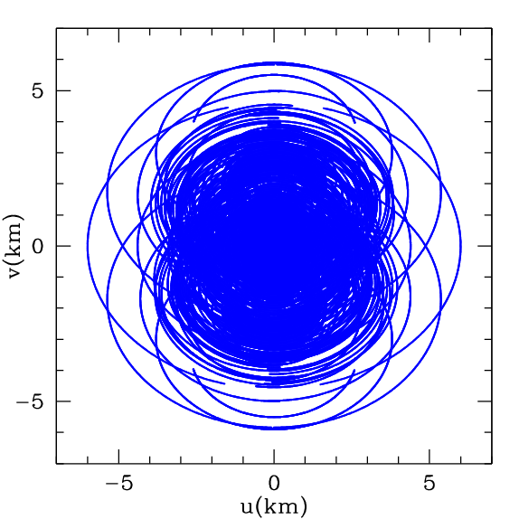
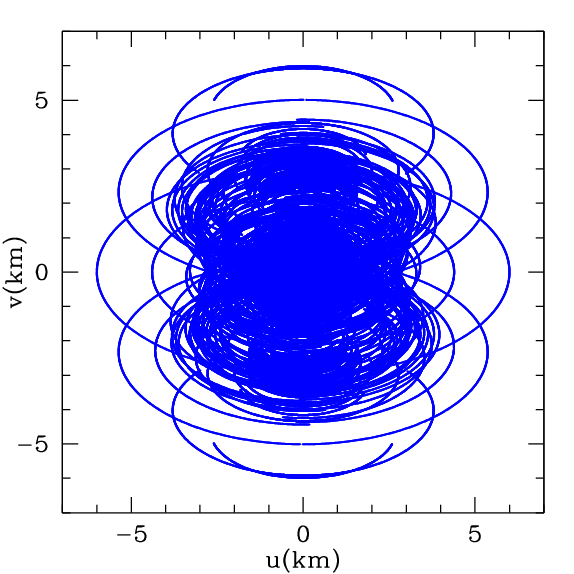
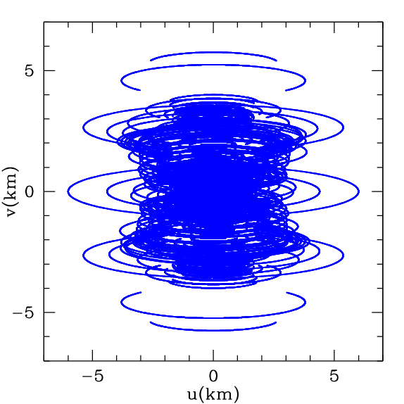
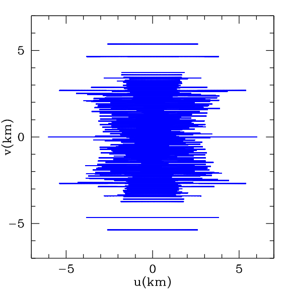
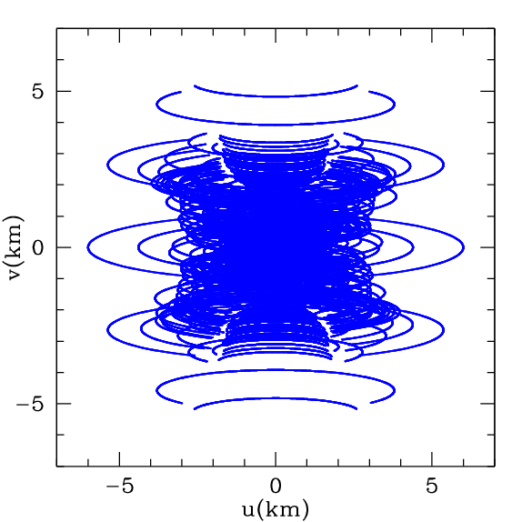
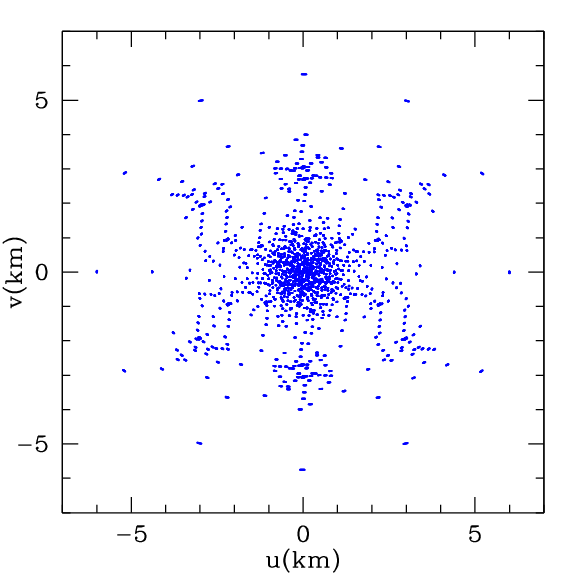
There are 630 baselines in the 36 antenna configuration for ASKAP. For illustrative purposes we show, in Figure 2, the UV coverage for a 10 hr track of a source at -50, -30, -10, 0 and +10 declination, and the snapshot (12 min) coverage for the same declinations in Figure 3. The frequency of the observation is 1.4 GHz and a narrow band (0.02 MHz) has been assumed (no multi-frequency synthesis).
 |
 |
 |
 |
 |
 |
 |
 |
 |
 |
 |
In Table 1 we summarise the size of the naturally weighted synthesised beam for different declinations and integration times. An elevation limit of 15 degrees was asummed for the antennas. Good circularity of the beam is maintained through a large declination range including declination 0 where currently much optical survey data is taken. The sidelobes levels of the beams are 3-4% over the entire declination range given in Table 1 except for ±3 degrees centered at declination 0. In this range the sidelobe levels get worse by a factor 2-3.
| Declination | Snapshot beam | 10 hr beam |
| (deg) | (arcsec x arcsec) | (arcsec x arcsec) |
| -50 | 19.1 x 15.4 | 19.4 x 15.9 |
| -30 | 17.6 x 15.2 | 18.9 x 17.5 |
| -10 | 17.9 x 15.3 | 19.6 x 18.2 |
| 0 | 18.4 x 15.3 | 19.5 x 19.3 |
| +10 | 21.5 x 15.1 | 20.1 x 19.2 |
| +30 | 26.5 x 15.3 | 26.1 x 16.8 |
| +40 | 31.6 x 16.5 | 31.2 x 16.5 |
Configuration Sensitivity
The sensitivity of the configuration at various angular scales is an important metric for ASKAP. The configuration is designed to optimise sensitivity on angular scales of 30" (for HI emission surveys; see Staveley-Smith 2006, 2008), whilst also providing good low surface brightness sensitivity (at low angular resolution) and high resolution imaging capability (see Condon 2007).
 |
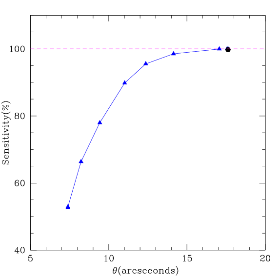 |
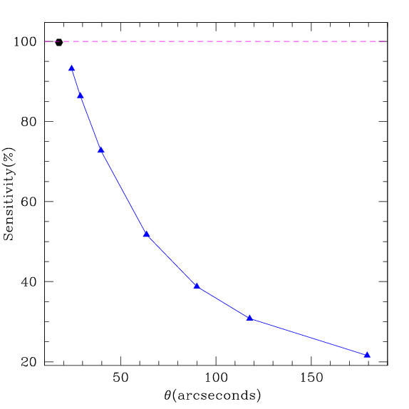
Left panel: Gaussian tapering of data was applied and results compared with the sensitivity obtained through natural weighting (solid black point). Right panel: Robust weighting was applied and the results compared with the sensitivity obtained through natural weighting (solid black point).
Sensitivity as a function of angular resolution is given in Figure 4, presented in two panels for clarity. The naturally weighted beam gives maximum sensitivity and an angular resolution of just under 20'' (see Table 1). This is indicated by the solid black point in Figure 4. Gaussian tapering was applied to the data with progressively larger and larger values, resulting in the curve shown in the left hand panel of Figure 4. In order to get higher resolution than that available with natural weighting it is necessary to downweight the short baselines at the expense of the longer baselines. This can be achieved through robust weighting (Briggs 2002) and the results are shown on the right hand panel of Figure 4.
Survey speeds and sensitivity for an interferometer like ASKAP have been derived elsewhere (e.g. Johnston & Gray 2006). To summarise, the time, t, required to reach a given sensitivity limit for point sources, σs , is

per second that can be surveyed to this sensitivity limit is
where F is the field of view in square degrees. The surface brightness temperature survey speed is given by

where now σt denotes the sensitivity limit in Kelvin and f relates to the filling factor of the array via
Here, εs is a `synthesised aperture efficiency' which is related to the weighting of the visibilities and is always ≤1.
In Table 2 we list values of the survey speed for different `typical' surveys for different angular resolutions. The first entry gives a continuum survey where the entire 300 MHz of bandwidth is exploited and a desired sensitivity (1-sigma) of 100 µJy is required. The second entry gives a spectral line survey, with the third line listing a surface brightness survey needing to reach 1K rms (1-sigma) over 5k Hz channel. Table 3 lists the sensitivity (1-sigma) after one hour of observation for the different surveys.
| Parameter | 10'' | 18'' | 30'' | 90'' | 180'' | units |
| Continuum survey speed (300 MHz, 100uJy) | 220 | 361 | 267 | 54 | 17 | sq deg/hr |
| Line survey speed (100kHz, 5mJy) | 184 | 301 | 223 | 45 | 14 | sq deg/hr |
| Surface brightness survey speed (5 kHz, 1K) | - | - | 1.1 | 18 | 94 | sq deg/hr |
| Parameter | 10'' | 18'' | 30'' | 90'' | 180'' | units |
| Continuum sensitivity (300 MHz) | 37 | 29 | 34 | 74 | 132 | µJy/bm |
| Line sensitivity (100 kHz) | 2.1 | 1.6 | 1.9 | 4.1 | 7.3 | mJy/bm |
| Surface brightness sensitivity (5 kHz) | 51 | 12 | 5.2 | 1.3 | 0.56 | K |
Hour Angle Coverage
The hour angle coverage as a function of declination for the ASKAP configuration (assuming an elevation limit of 15 degrees for the antennas) is shown in Figure 5. South of declination 0, a minimum of 10 hour tracks are possible. At declinations +10, +20, +30 and +40 maximum time above the horizon is 9.0, 8.0, 6.9 and 4.9 hours respectively. Shadowing may occur on some baselines for some combinations of declinations and hour angles.
 |
Notes
A full site survey has not yet been carried out at time of writing (October 2008). Results from the site survey may alter the position of some of the antennas in this layout. The system temperature and aperture efficiency are still not well determined but should become better known towards the middle of 2009.
Acknowledgments
We thank Robert Braun, Jim Condon and Lister Staveley-Smith for useful discussions and contributions. We acknowledge the use of casapy for our simulations.
References
Ball, L., 2008, ATNF Science in 2010-2015.
Briggs, D., 2002, PhD Thesis
Condon, J., 2008, ATNF SKA Memo Series, 015
de Villiers M., 2007, A&A, 469, 793
Feain, I., Johnston, S., Gupta, N., ATNF SKA Memo Series, 017
Gupta, N., Johnston, S., Feain, I., ATNF SKA Memo Series, 016
Johnston S. et al., 2007, PASA, 24, 174
Johnston et al. 2008, Experimental Astronomy, In Press
Staveley-Smith L., 2006, ATNF SKA Memo Series, 006
Staveley-Smith L., 2008, ATNF SKA Memo Series, 020
Further Information
For more information on ASKAP science activities contact the ASKAP Project Scientist.