If we average all the channels in the band together, then we must assign a single frequency and a single (u,v) coordinate to each visibility. Clearly this means a loss of information, because u and v change across the band (they are the orthogonal baseline components measured in wavelengths in the plane perpendicular to the direction of the source, with v in the northern direction).
The simplest way to understand the effect upon the final image is via
the similarity theorem of Fourier transforms, which states that if ![]() and
and ![]() are a Fourier pair in n dimensions,
then rescaling the coordinates in one domain by a factor of
are a Fourier pair in n dimensions,
then rescaling the coordinates in one domain by a factor of ![]() corresponds to rescaling the transform by the reciprocal scale factor, and
renormalizing the amplitudes such that
corresponds to rescaling the transform by the reciprocal scale factor, and
renormalizing the amplitudes such that
![]()
In our case, we associate the visibilities (V) with h and the image (I)
with H. Thus, we measure a visibility V(u,v) at some frequency ![]() in
the band, and then scale its coordinates to
in
the band, and then scale its coordinates to ![]() (appropriate to the frequency at the centre of the band) such that
(appropriate to the frequency at the centre of the band) such that
![]()
The similarity theorem shows that the image made from visibilities that have
been scaled in this way is stretched and scaled such that the contribution to
the visibility from a narrow band of frequencies centered on ![]() is
is
![]()
where l and m are the image coordinates (direction cosines). Each
image is the true brightness distribution scaled in (l,m) by ![]() and
in brightness by
and
in brightness by ![]() . The derived distribution is convolved by the
dirty beam
. The derived distribution is convolved by the
dirty beam ![]() . The beam does not vary with frequency because the
same transfer function for the telescope (i.e., the sampling of the array in
the
. The beam does not vary with frequency because the
same transfer function for the telescope (i.e., the sampling of the array in
the ![]() plane) is used to represent the whole frequency passband. The
overall response over the whole band is simply obtained by integrating over the
passband with the appropriate weighting.
plane) is used to represent the whole frequency passband. The
overall response over the whole band is simply obtained by integrating over the
passband with the appropriate weighting.
![]()
where ![]() is the passband function. This integral can be thought of
as a process of averaging many images, each with a different scale factor.
The images are aligned at the phase centre, so that the effect is to produce
a radial smearing of the brightness distribution (and consequent
loss of intensity) before it is convolved with the beam. The response to a
point source at position (l,m) is radially elongated by the factor
is the passband function. This integral can be thought of
as a process of averaging many images, each with a different scale factor.
The images are aligned at the phase centre, so that the effect is to produce
a radial smearing of the brightness distribution (and consequent
loss of intensity) before it is convolved with the beam. The response to a
point source at position (l,m) is radially elongated by the factor ![]() . For distances from the origin at which the elongation
is large compared to the synthesized beamwidth, features on the sky become
suppressed by the smearing; the integrated flux density remains unchanged, but
the surface brightness is reduced. The measured brightness is the smeared
distribution convolved by the beam.
. For distances from the origin at which the elongation
is large compared to the synthesized beamwidth, features on the sky become
suppressed by the smearing; the integrated flux density remains unchanged, but
the surface brightness is reduced. The measured brightness is the smeared
distribution convolved by the beam.
It turns out that the results are only weakly dependent on parameters such as
the exact passband shape and beam shape, so, as a good example, the figure shows
the relative amplitude of the peak response to a point source as a function of
distance from the field centre (r), the beamwidth (![]() ), and
fractional bandwidth (
), and
fractional bandwidth (![]() ). It can be used to determine
whether your data will suffer too badly should you average across the band.
As a rough guide, you probably don't want to accept a bandwidth that
results in an amplitude drop to less than
). It can be used to determine
whether your data will suffer too badly should you average across the band.
As a rough guide, you probably don't want to accept a bandwidth that
results in an amplitude drop to less than ![]() .
.
Note that since the AT always produces spectral data, you are free to average channels in any combination you choose. You are not restricted to averaging the whole band and might desire to average it into three sections say, none of which suffers from bandwidth smearing.
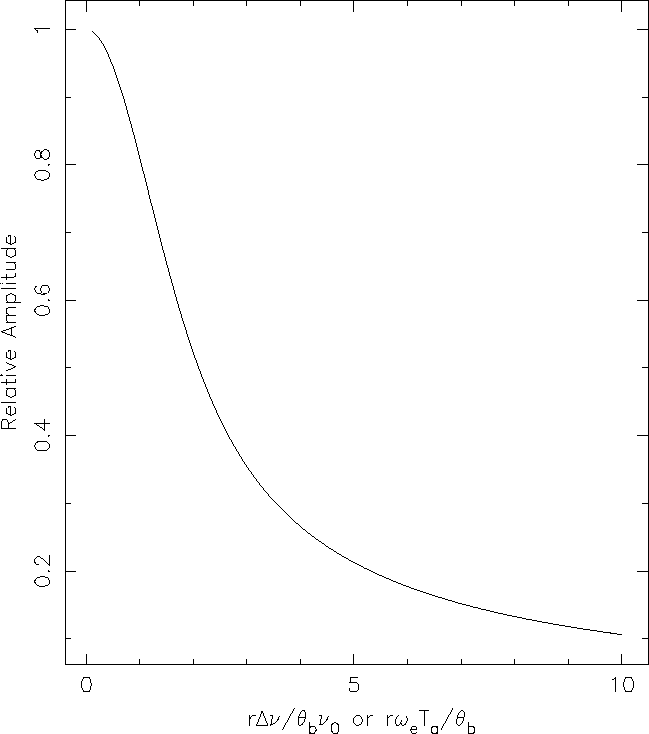
Figure: Relative amplitude of the peak response to a point source
as a function of the distance from the field centre and either the
fractional bandwidth or the averaging time