Direction-Dependent Calibration
YANDASoft has a new direction-dependent (DD) calibration application, cddcalibrator. While this application and the associated solver are still under development, this user recipe will be updated with examples of how to setup and use the solver.
Quick Algorithm Overview
Normal equation setup (single calibration direction)
Model visibility: Mij(t,f) = gigj* Iij(t,f)
Measured visibility: Vij(t,f) = (gi+ ei) (gj+ ej)* Iij(t,f) + noise
Residual visibility: Rij(t,f) ~ giIij(t,f) ej* + gj* Iij(t,f) ei + noise
r = A e
e = (A’ A)-1A’ r
iterate
e = (A’ A)-1(A’ v - A’ m)
The gain terms can be factored out of the A’ A and A’ v matrices, which contain all of the averaging in time and frequency, so they can be pre-calculated and used to form the normal equations inside the convergence loop.
Can include other directions as extra matrix blocks, and can subtract extra A m terms rather than coupling the blocks.
e1 = (A1‘ A1)-1(A1' v - A1 m1- A1‘ m2- A1‘ m3- …)
Simulating test data
An array configuration file is needed for the simulation. For this, the SKA1-LOW core stations from SKA document, SKA-TEL-SKO-0000422_03_SKA1_LowConfigurationCoordinates.txt, were used and converted to standard global X,Y,Z coordinates. Restricting the simulation to the core was for some simple ionospheric calibration tests, and also to keep some imaging tests at low resolution:
antennas.telescope = SKA1_Low
antennas.SKA1_Low.coordinates = global
antennas.SKA1_Low.names = [C1,C2,C3,C4,C5,C6,C7,C8,C9,C10,C11,C12,C13,C14,C15,C16,C17,C18,C19,C20,C21,C22,C23,C24,C5,C26,C27,C28,C29,C30,C31,C32,C33,C34,C35,C36,C37,C38,C39,C40,C41,C42,C43,C44,C45,C46,C47,C48,C49,C50,C51,C52,C53,C54,C55,C56,C57,C58,C59,C60,C61,C62,C63,C64,C65,C66,C67,C68,C69,C70,C71,C72,C73,C74,C75,C76,C77,C78,C79,C80,C81,C82,C83,C84,C85,C86,C87,C88,C89,C90,C91,C92,C93,C94,C95,C96,C97,C98,C99,C100,C101,C102,C103,C104,C105,C106,C107,C108,C109,C110,C111,C112,C113,C114,C115,C116,C117,C118,C119,C120,C121,C122,C123,C124,C125,C126,C127,C128,C129,C130,C131,C132,C133,C134,C135,C136,C137,C138,C139,C140,C141,C142,C143,C144,C145,C146,C147,C148,C149,C150,C151,C152,C153,C154,C155,C156,C157,C158,C159,C160,C161,C162,C163,C164,C165,C166,C167,C168,C169,C170,C171,C172,C173,C174,C175,C176,C177,C178,C179,C180,C181,C182,C183,C184,C185,C186,C187,C188,C189,C190,C191,C192,C193,C194,C195,C196,C197,C198,C199,C200,C201,C202,C203,C204,C205,C206,C207,C208,C209,C210,C211,C212,C213,C214,C215,C216,C217,C218,C219,C220,C221,C222,C223,C224]
antennas.SKA1_Low.diameter = 35.0m
antennas.SKA1_Low.C1 = [-2563226.960308, 5081884.949807, -2878357.951618]
antennas.SKA1_Low.C2 = [-2563113.882419, 5082069.138800, -2878133.437661]
antennas.SKA1_Low.C3 = [-2563205.012109, 5081946.412641, -2878268.979042]
...
antennas.SKA1_Low.C224 = [-2563323.596627, 5081739.381914, -2878528.892342]
A gain corruption file is also needed. This was generate randomly with 10% Gaussian noise added to ideal gains of 1+0i. Corruption file gains.core.field1.true is:
gain.g11.0.0  = [0.851337,0.102628]
gain.g11.1.0  = [0.910252,-0.010673]
gain.g11.2.0  = [1.157664,0.184521]
...
gain.g11.223.0  = [1.055898,0.058924]

gain.g22.0.0  = [0.851337,0.102628]
gain.g22.1.0  = [0.910252,-0.010673]
gain.g22.2.0  = [1.157664,0.184521]
...
gain.g22.223.0  = [1.055898,0.058924]
The parameter format is:
<parameter type (gain, leakage, etc.)>.<polarisation (g11, g22, d12, d21)>.<antenna>.<beam (aka direction for DD calibration)>.
We can now simulate visibilities for one of the calibration directions. After some of the recent work, it may be possible to generate multiple fields with different gain corruptions in a single csimulator run, but this needs to be tested. As in the sky model sections below, the simulation sky model can be defined via comopnents or images. Here components are used. The csimulator parset file for this direction is:
Csimulator.dataset                     = vis_field1.ms

Csimulator.sources.names               = [field1]
Csimulator.sources.field1.direction    = [12h30m00.0,-45.00.00.0,J2000]
Csimulator.sources.field1.components   = [comp1,comp2]
Csimulator.sources.comp1.direction.ra  =  0.06
Csimulator.sources.comp1.direction.dec = -0.02
Csimulator.sources.comp1.flux.i        = 1.0
Csimulator.sources.comp2.direction.ra  =  0.05
Csimulator.sources.comp2.direction.dec = -0.024
Csimulator.sources.comp2.flux.i        = 1.0

Csimulator.noise                       = false
Csimulator.noise.rms                   = 1

Csimulator.corrupt                     = true
Csimulator.calibaccess                 = parset
Csimulator.calibaccess.parset          = gains.core.field1.true

Csimulator.antennas.definition         = SKA-TEL-SKO-0000422_03_SKA1_LowConfig_core.in

Csimulator.feeds.names                 = [feed0]
Csimulator.feeds.feed0                 = [0.0, 0.0]

Csimulator.spws.names                  = [SPW]
Csimulator.spws.SPW                    = [3, 150.0MHz, -1MHz, "XX XY YX YY"]

Csimulator.simulation.blockage         = 0.0
Csimulator.simulation.elevationlimit   = 0deg
Csimulator.simulation.autocorrwt       = 0.0
Csimulator.simulation.usehourangles    = True
Csimulator.simulation.referencetime    = [2015June24, UTC]

Csimulator.simulation.integrationtime  = 1s

Csimulator.observe.number              = 1
Csimulator.observe.scan0               = [field1, SPW, 0s, 5s]

Csimulator.gridder                     = SphFunc
The csimulator parset file for a second direction is the same, except for the following parameters:
Csimulator.dataset                           = vis_field2.ms

Csimulator.sources.names                     = [field2]
Csimulator.sources.field2.direction          = [12h30m00.0,-45.00.00.0,J2000]
Csimulator.sources.field2.components         = [comp1,comp2,comp3]
Csimulator.sources.comp1.direction.ra        = -0.05
Csimulator.sources.comp1.direction.dec       =  0.08
Csimulator.sources.comp1.flux.i              = 1.0
Csimulator.sources.comp1.flux.spectral_index = -0.2
Csimulator.sources.comp1.flux.ref_freq       = 200e6
Csimulator.sources.comp2.direction.ra        = -0.039
Csimulator.sources.comp2.direction.dec       =  0.081
Csimulator.sources.comp2.flux.i              = 0.6
Csimulator.sources.comp2.flux.spectral_index = -0.73
Csimulator.sources.comp2.flux.ref_freq       = 200e6
Csimulator.sources.comp2.shape.bmaj          = 0.001309
Csimulator.sources.comp2.shape.bmin          = 0.001091
Csimulator.sources.comp2.shape.bpa           = 1.855
Csimulator.sources.comp3.direction.ra        = -0.051
Csimulator.sources.comp3.direction.dec       =  0.074
Csimulator.sources.comp3.flux.i              = 1.3
Csimulator.sources.comp3.flux.spectral_index = -0.75
Csimulator.sources.comp3.flux.ref_freq       = 200e6
Csimulator.sources.comp3.shape.bmaj          = 1.164e-3
Csimulator.sources.comp3.shape.bmin          = 1.091e-3
Csimulator.sources.comp3.shape.bpa           = 1.205

Csimulator.calibaccess.parset                = gains.core.field2.true

Csimulator.observe.scan0                     = [field2, SPW, 0s, 5s]
Corruption file gains.core.field2.true has the same 10% deviations as the first, but additional distortions at the 1% level. The two simulation parsets are processed by csimulator:
csimulator -c parset_field1.in > parset_field1.log
csimulator -c parset_field2.in > parset_field2.log
Both the simulator and the calibrator can be run in parallel across frequency and/or Taylor term, as described in csimulator and cddcalibrator. The resulting measurement sets added together using a casa script, e.g. using casapy -- -c merge.py for merge.py file:
# first:
# cp -r vis_field1.ms vis_2fields.ms

tb.open("vis_field1.ms")
data1=tb.getcol("DATA");
tb.close()
tb.open("vis_field2.ms")
data2=tb.getcol("DATA");
tb.close()
for i in range(len(data1)):
    for j in range(len(data1[0])):
        for k in range(len(data1[0][0])):
            data1[i][j][k] = data1[i][j][k] + data2[i][j][k]
tb.open("vis_2fields.ms", nomodify=False)
tb.putcol("DATA", data1);
tb.close()
Current Limitations
Components were added to yandasoft for debugging and testing purposes, and as such are not as flexible as might be desired. The baseline design is an image-based sky model, with multiple planes for polarisation and frequency (or separate Taylor term images) and A-projection for the primary beam response. Some current limitations are:
The sources.comp11.direction.ra and dec parameters are actually l and m coordinates. Should support ra,dec and l,m options.
Multiple sources.fieldname.direction parameters are not supported. The first is used to set the phase centre of the measurement set, and all l,m coordinates are set relative to that.
Components are not at present multiplied by the primary beam.
There is no polarisation or Faraday rotation.
DD-cal with component-based sky models
To generate calibration solutions for the combined measurement set, the new application cddcalibrator is used. An example parset for this is:
Cddcalibrator.dataset                            = vis_2fields.ms

Cddcalibrator.sources.names                      = [field1,field2]

Cddcalibrator.sources.field1.direction           = [12h30m00.000, -45.00.00.000, J2000]
Cddcalibrator.sources.field1.components          = [comp11,comp12]
Cddcalibrator.sources.comp11.direction.ra        =  0.06
Cddcalibrator.sources.comp11.direction.dec       = -0.02
Cddcalibrator.sources.comp11.flux.i              = 1.0
Cddcalibrator.sources.comp12.direction.ra        =  0.05
Cddcalibrator.sources.comp12.direction.dec       = -0.024
Cddcalibrator.sources.comp12.flux.i              = 1.0

Cddcalibrator.sources.field2.direction           = [12h30m00.0,-45.00.00.0,J2000]
Cddcalibrator.sources.field2.components          = [comp21,comp22,comp23]
Cddcalibrator.sources.comp21.direction.ra        = -0.05
Cddcalibrator.sources.comp21.direction.dec       =  0.08
Cddcalibrator.sources.comp21.flux.i              = 1.0
Cddcalibrator.sources.comp21.flux.spectral_index = -0.2
Cddcalibrator.sources.comp21.flux.ref_freq       = 200e6
Cddcalibrator.sources.comp22.direction.ra        = -0.039
Cddcalibrator.sources.comp22.direction.dec       =  0.081
Cddcalibrator.sources.comp22.flux.i              = 0.6
Cddcalibrator.sources.comp22.flux.spectral_index = -0.73
Cddcalibrator.sources.comp22.flux.ref_freq       = 200e6
Cddcalibrator.sources.comp22.shape.bmaj          = 0.001309
Cddcalibrator.sources.comp22.shape.bmin          = 0.001091
Cddcalibrator.sources.comp22.shape.bpa           = 1.855
Cddcalibrator.sources.comp23.direction.ra        = -0.051
Cddcalibrator.sources.comp23.direction.dec       =  0.074
Cddcalibrator.sources.comp23.flux.i              = 1.3
Cddcalibrator.sources.comp23.flux.spectral_index = -0.75
Cddcalibrator.sources.comp23.flux.ref_freq       = 200e6
Cddcalibrator.sources.comp23.shape.bmaj          = 1.164e-3
Cddcalibrator.sources.comp23.shape.bmin          = 1.091e-3
Cddcalibrator.sources.comp23.shape.bpa           = 1.205

Cddcalibrator.solve                              = gains
Cddcalibrator.solver                             = LSQR
Cddcalibrator.ncycles                            = 25

Cddcalibrator.nAnt                               = 224
Cddcalibrator.nChan                              = 1
Cddcalibrator.nCal                               = 2

Cddcalibrator.refantenna                         = 1

Cddcalibrator.gridder                            = SphFunc

Cddcalibrator.calibaccess                        = parset
Cddcalibrator.calibaccess.parset                 = cddcal_components.out
This can be processed using cddcalibrator:
cddcalibrator -c parset_components.in > parset_components.log
With a resulting calibration parset:
gain.g11.0.0 = [0.850075,0.112602]
gain.g11.0.1 = [0.85372,0.0998866]
gain.g11.1.0 = [0.910315,0]
gain.g11.1.1 = [0.915879,0]
gain.g11.2.0 = [1.15542,0.198081]
gain.g11.2.1 = [1.14571,0.182439]
gain.g11.3.0 = [1.10343,-0.0382154]
gain.g11.3.1 = [1.12954,-0.0492568]
...
gain.g11.223.0 = [1.03577,0.152637]
gain.g11.223.1 = [1.02706,0.132094]

gain.g22.0.0 = [0.912248,-0.213603]
gain.g22.0.1 = [0.893442,-0.223309]
gain.g22.1.0 = [1.05976,0]
gain.g22.1.1 = [1.08265,0]
gain.g22.2.0 = [0.880054,0.00892662]
gain.g22.2.1 = [0.891396,-0.00518362]
gain.g22.3.0 = [1.01041,-0.0441419]
gain.g22.3.1 = [0.993966,-0.0422119]
...
gain.g22.223.0 = [1.05073,-0.11987]
gain.g22.223.1 = [1.02655,-0.105639]
If the true gain corruptions are also phase referenced to the second antenna, they agree closely with the calibration results:
first direction:
gain.g11.0.0  = 0.8500752+0.1126024j
gain.g11.1.0  = 0.9103145-0j
gain.g11.2.0  = 1.1554210+0.1980813j
gain.g11.3.0  = 1.1034349-0.0382153j
...
gain.g11.223.0  = 1.0357685+0.1526373j

gain.g22.0.0  = 0.9122477-0.2136029j
gain.g22.1.0  = 1.0597603-0j
gain.g22.2.0  = 0.8800543+0.0089266j
gain.g22.3.0  = 1.0104071-0.0441418j
...
gain.g22.223.0  = 1.0507253-0.1198698j

second direction:
gain.g11.0.0  = 0.8537200+0.0998865j
gain.g11.1.0  = 0.9158786-0j
gain.g11.2.0  = 1.1457061+0.1824390j
gain.g11.3.0  = 1.1295440-0.0492567j
...
gain.g11.223.0  = 1.0270592+0.1320941j

gain.g22.0.0  = 0.8934421-0.2233087j
gain.g22.1.0  = 1.0826515+0j
gain.g22.2.0  = 0.8913956-0.0051836j
gain.g22.3.0  = 0.9939656-0.0422119j
...
gain.g22.223.0  = 1.0265463-0.1056391j
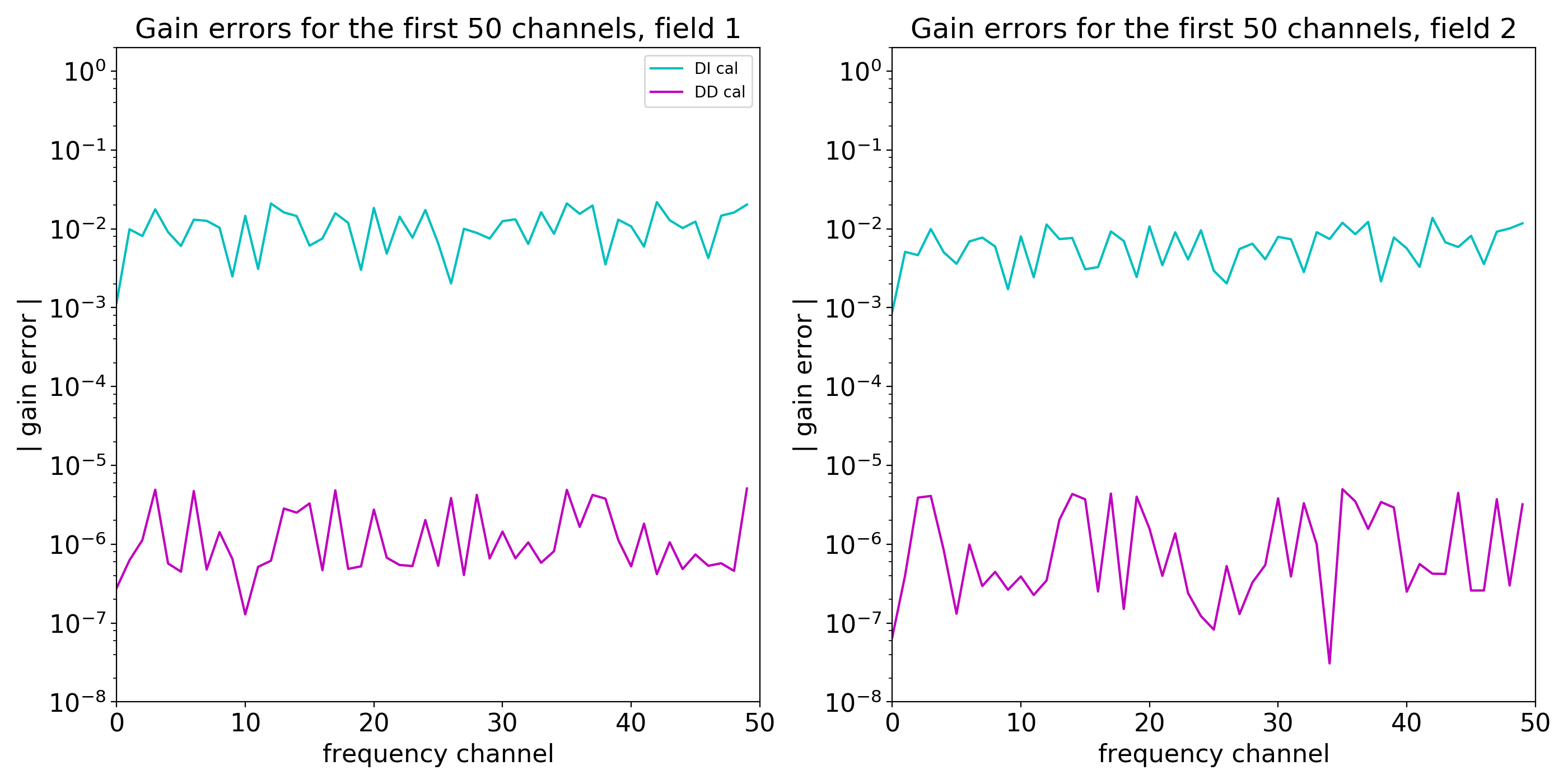
The calibration errors are shown in the following figure. Also shown are the errors after direction-independent calibration using a sky model that contains all five comopnents.
Current Limitations
Much the same as for component-based simulations above. Some specific issues are:
The sources.fieldname.direction parameter is currently ignored. The phase centre of the measurement set is used.
DD-cal with image-based sky models
Simulation and calibration parset files for image-based sky models are much the same as those for component-based sky models, except, of course, for the *.sources.* parameters, but also in general for the gridders used to degrid the images.
Sky models can be pre-existing images – an image of clean components, for instance – or they can be generated from a list of components using the cmodel application. Cmodel can read a number of different database types, such as a votable, a GSM dataservice, or an user-defined asciitable. See cmodel for all of the options.
To redo the steps above but this time with image-based models, first a cmodel parset file for each direction:
# GSM parameters
Cmodel.gsm.database                    = asciitable
Cmodel.gsm.file                        = cmodel_field1.cat
Cmodel.gsm.ref_freq                    = 200MHz

# asciitable format parameters
Cmodel.tablespec.ra.col                = 1
Cmodel.tablespec.ra.units              = deg
Cmodel.tablespec.dec.col               = 2
Cmodel.tablespec.dec.units             = deg
Cmodel.tablespec.flux.col              = 3
Cmodel.tablespec.flux.units            = Jy
Cmodel.tablespec.majoraxis.col         = 4
Cmodel.tablespec.majoraxis.units       = arcmin
Cmodel.tablespec.minoraxis.col         = 5
Cmodel.tablespec.minoraxis.units       = arcmin
Cmodel.tablespec.posangle.col          = 6
Cmodel.tablespec.posangle.units        = deg
Cmodel.tablespec.spectralindex.col     = 7
Cmodel.tablespec.spectralindex.units   = Jy

# output parameters
Cmodel.bunit                           = Jy/pixel
Cmodel.frequency                       = 200MHz
Cmodel.increment                       = 1MHz
Cmodel.flux_limit                      = 10uJy

# image parameters
Cmodel.shape                           = [1024,1024]
Cmodel.cellsize                        = [51.6arcsec, 51.6arcsec]
Cmodel.direction                       = [12h30m00.000, -45.00.00.000, J2000]
Cmodel.stokes                          = [I]
Cmodel.nterms                          = 3
Cmodel.output                          = casa
Cmodel.filename                        = image.field1
The catalogue file, cmodel_field1.cat, contains the two components for field1, converted from (1,m) coordinates to (ra,dec) coordinates:
comp1 192.458664 -46.040718 1.00 0.0 0.0 0.0 0.0
comp2 191.650331 -46.301810 1.00 0.0 0.0 0.0 0.0
And similarly for field2:
comp1 183.738540 -40.344699 1.0 0.000000 0.000000 0.000000 -0.20
comp2 184.568249 -40.313384 0.6 4.500010 3.750582 106.2837 -0.73
comp3 183.643561 -40.686476 1.3 4.001537 3.750582 69.04141 -0.75
For each field this will create three images, e.g. “mpirun -np 2 cmodel -c cmodel_field1.in > cmodel_field1.log” produces: image.field1.taylor.0, image.field1.taylor.1 and image.field1.taylor.2.
These can then be used in csimulator in place of the components, e.g.:
Csimulator.sources.names            = [field1]
Csimulator.sources.field1.direction = [12h30m00.000, -45.00.00.000, J2000]
Csimulator.sources.field1.model     = [image.field1.taylor.0,image.field1.taylor.1]
Csimulator.sources.field1.nterms    = 2
And also for cddcalibrator:
Cddcalibrator.sources.names            = [field1,field2]

Cddcalibrator.sources.field1.direction = [12h30m00.0,-45.00.00.0,J2000]
Cddcalibrator.sources.field1.model     = [image.field1.taylor.0,image.field1.taylor.1]
Cddcalibrator.sources.field1.nterms    = 2

Cddcalibrator.sources.field2.direction = [12h30m00.0,-45.00.00.0,J2000]
Cddcalibrator.sources.field2.model     = [image.field2.taylor.0,image.field2.taylor.1]
Cddcalibrator.sources.field2.nterms    = 2
Current Limitations
Different directions can be specified for each field, however the model visibilities generated for calibration are phase centred in these directions. An extra rotation of the models will be needed to have a small offset image for each field.
The order of fields seems to be sorted, which complicates the interpretation of the output calibration files.
Work in progress and next steps
New normal equation structure to solve low-order phase functions across the aperture.
Demonstrations on precursor datasets and more realistic simulations.
Use regularised solver to couple solutions across directions
The current setup uses pre-averaged calibration matrices to avoid full regeneration of the normal equation every iteration of the solver. However this may not be the best match for short ionospheric calibration intervals, as there are extra overheads for multiple directions.
The DD calibration extensions have not be profiled and optimised at this point. The focus has been on accuracy rather than performance.