Direction-Dependent Ionospheric Calibration

YANDASoft has a new direction-dependent (DD) calibration application, cddcalibrator. While this application and the associated solver are still under development, this user recipe will be updated with examples of how to setup and use the solver.

Quick Algorithm Overview

Normal equation setup (single calibration direction)

Model visibility:

\[M_{ij} = g_i g_j^* I_{ij} \exp( -2\pi (u_{ij}l + v_{ij}m + w_{ij}n) )\]

Measured visibility:

\[V_{ij} = M_{ij} \exp( -2\pi i \lambda^2 (u_{ij}'\alpha_l + v_{ij}'\alpha_m) ) + \mbox{noise}\]

\[V_{ij} = M_{ij} (1 - 2\pi i \lambda^2 (u_{ij}'\alpha_l + v_{ij}'\alpha_m) + \mbox{higher order terms} ) + \mbox{noise}\]

Residual visibility:

\[R_{ij} = M_{ij} (-2\pi i \lambda^2 (u_{ij}'\alpha_l + v_{ij}'\alpha_m) + \mbox{higher order terms} ) + \mbox{noise}\]

Standard least squares:

• r = A e

• e = (A’ A)^-1A’ r

• iterate

e = (A’ A)^-1(A’ v - A’ m)

• The (u’,v’) coordinates can simply be the standard (u,v) coordinates, however they are not limited to this. For instance, they could be x_i- x_j and y_i- y_j coordinates in the local horizontal coordinate system, in which case the ionosphere would be modelled in a plane parallel to the array. This is the current approach used in cddcalibrator.

• The α-terms describe a linear phase gradient across the aperture for this direction, equivalent to a frequency-dependent position shift. This generally will only be appropriate for apertures of a few kilometres.

• Extending to high orders can be achieved using functions other than (u’,v’), in which case the effect of the ionosphere can no longer be thought of as a frequency-dependent position shift. For instance, first and second order Zernike polynomials defined within a circular aperture could be used in a straighforward manner.

• Though not currently implemented, a combination of α-terms, β-terms, etc., could be combined with station-based DTEC terms. Restricting the aperture function to the inner part of the array could be a useful way to limit the number of aperture coefficients while also limiting the number of free parameters in antenna-based calibration.

• The α-terms can be factored out of the A’ A and A’ v matrices, which contain all of the averaging in time, so they can be pre-calculated and used to form the normal equations inside the convergence loop.

• Can include other directions as extra matrix blocks, and can subtract extra A m terms rather than coupling the blocks.

• e₁ = (A₁‘ A₁)^-1(A₁' v - A₁ m₁- A₁‘ m₂- A₁‘ m₃- …)

DD-cal with component-based sky models

Test data can be simulated following a similar approach to the Direction-Dependent Calibration user recipe. However, due to the frequency dependence of the ionosphere, simulating linear position shifts would need to be done separately for each frequency channel. These data can then be merged using msmerge (Measurement Merging Utility).

For the processing below, field1 was generated with an offset of [+1”,-2”] at a wavelength of 2m, resulting in coefficients of [7.27e-5,-1.45e-4] rad/m^2. Field2 was generated with an offset of [-3”,0”] at a wavelength of 2m, resulting in coefficients of [-2.18e-4,0.00] rad/m^2.

To generate calibration solutions for the combined measurement set, the new application cddcalibrator is used. An example parset for this is:

Cddcalibrator.dataset                            = vis_2fields.ms

Cddcalibrator.sources.names                      = [field1,field2]

Cddcalibrator.sources.names                        = [field1,field2]
Cddcalibrator.sources.field1.direction             = [12h30m00.000, -45.00.00.000, J2000]
Cddcalibrator.sources.field1.components            = [comp1]
Cddcalibrator.sources.comp1.flux.i                  = 1.0
Cddcalibrator.sources.comp1.direction.ra            =  0.06
Cddcalibrator.sources.comp1.direction.dec           = -0.02
Cddcalibrator.sources.field2.direction             = [12h30m00.000, -45.00.00.000, J2000]
Cddcalibrator.sources.field2.components            = [comp2]
Cddcalibrator.sources.comp2.flux.i                  = 0.5
Cddcalibrator.sources.comp2.direction.ra            = -0.06
Cddcalibrator.sources.comp2.direction.dec           =  0.08

Cddcalibrator.frequencies                          = [3, 150.0MHz, -1MHz]
Cddcalibrator.antennas.definition                  = SKA-TEL-SKO-0000422_03_SKA1_LowConfig_core.in

Cddcalibrator.solve                              = ionosphere
Cddcalibrator.solver                             = LSQR
Cddcalibrator.ncycles                            = 25

Cddcalibrator.nAnt                               = 224
Cddcalibrator.nChan                              = 3
Cddcalibrator.nCal                               = 2

Cddcalibrator.gridder                            = SphFunc

Cddcalibrator.calibaccess                        = parset
Cddcalibrator.calibaccess.parset                 = cddcal_components.out

This can be processed using cddcalibrator:

cddcalibrator -c parset_components.in > parset_components.log

With a resulting calibration parset:

ionosphere.linear.0.0 = [7.4235e-05,0]
ionosphere.linear.1.0 = [-0.000135432,0]
ionosphere.linear.0.1 = [-0.000217818,0]
ionosphere.linear.1.1 = [2.74816e-06,0]

with the first index indicating the α-term and the second indication the direction.

Simulated SKA1-LOW Data

Obtain the short EoR0 observation with GLEAM sources:

gsutil -m cp -r gs://ska1-simulation-data/ska1-low/direction_dependent_sims_SP-1056/SKA_LOW_SIM_short_EoR0_ionosphere_off_GLEAM.MS .

gsutil -m cp -r gs://ska1-simulation-data/ska1-low/direction_dependent_sims_SP-1056/SKA_LOW_SIM_short_EoR0_ionosphere_on_GLEAM.MS .

Although we know which columns of the GLEAM catalogue were used in the simulations, the yandasoft calibration classes are not yet connected to the primary beam models used in the simulations. This will be implemented soon, but for now the flux density of sources are estimated from an image of the data without ionospheric distortions. For a synthesised beam resolution of about 5.5’, the following was used:

Cimager.dataset                          = SKA_LOW_SIM_short_EoR0_ionosphere_off_GLEAM.MS
Cimager.nUVWMachines                     = 1
Cimager.uvwMachineDirTolerance           = 1arcsec
Cimager.imagetype                        = casa
Cimager.memorybuffers                    = true

Cimager.Images.Names                     = [image.short_EoR0_ionosphere_off]
Cimager.Images.shape                     = [8192,8192]
Cimager.Images.cellsize                  = [1.82arcsec, 1.82arcsec]

Cimager.gridder                          = WProject
Cimager.gridder.WProject.nwplanes        = 99
Cimager.gridder.WProject.oversample      = 8
Cimager.gridder.WProject.maxsupport      = 1024
Cimager.gridder.WProject.cutoff          = 0.001
Cimager.gridder.WProject.variablesupport = true

Cimager.solver                           = Clean
Cimager.solver.Clean.algorithm           = Hogbom
Cimager.solver.Clean.niter               = 100
Cimager.solver.Clean.gain                = 0.1
Cimager.solver.Clean.tolerance           = 0.01
Cimager.solver.Clean.verbose             = True
Cimager.threshold.minorcycle             = [10%]

Cimager.ncycles                          = 5

Cimager.restore                          = True
Cimager.restore.beam                     = fit

Cimager.preconditioner.preservecf        = true
Cimager.preconditioner.Names             = [Wiener]
Cimager.preconditioner.Wiener.robustness = -2

For the widely separated brighter sources, there is not much benefit in fitting them in a joint, peeling setup. To processes them separately, the following parsets were used.

Common parameters:

# only interested in the core antennas, so I flagged all
# stations above number 224, and all baselines longer than 1km.
Cddcalibrator.dataset             = SKA_LOW_SIM_short_EoR0_ionosphere_on_GLEAM_flagged.MS
Cddcalibrator.solve               = ionosphere
Cddcalibrator.solver              = LSQR
Cddcalibrator.ncycles             = 10
Cddcalibrator.interval            = 1s

# parameters need for the ionospheric algorithm
Cddcalibrator.frequencies         = [11, 125MHz, 5MHz]
Cddcalibrator.antennas.definition = SKA_LOW_SIM_Config_local.in

# even though there is only 1 solution for the whole band,
# the buffers need to fit all of the channels
Cddcalibrator.nAnt                = 512
Cddcalibrator.nChan               = 11
Cddcalibrator.nCal                = 1

# do not need a gridder when using component sky models, but need to specify something
Cddcalibrator.gridder             = SphFunc

Parameters for radio source J000045-272248 (and close neighbour J000019-272511):

Cddcalibrator.sources.names                        = [cal1]
Cddcalibrator.sources.cal1.direction               = [00h00m00.000, -27.00deg, J2000]
Cddcalibrator.sources.cal1.components              = [J000045-272248,J000019-272511]
Cddcalibrator.sources.J000045-272248.flux.i        = 2.855 # from uncorrupted image
Cddcalibrator.sources.J000045-272248.direction.ra  = +0.002929
Cddcalibrator.sources.J000045-272248.direction.dec = -0.006636
Cddcalibrator.sources.J000019-272511.flux.i        = 0.59
Cddcalibrator.sources.J000019-272511.direction.ra  = +0.001248
Cddcalibrator.sources.J000019-272511.direction.dec = -0.007328

Parameters for radio source J000217-253912:

Cddcalibrator.sources.names                        = [cal2]
Cddcalibrator.sources.cal2.direction               = [00h00m00.000, -27.00deg, J2000]
Cddcalibrator.sources.cal2.components              = [J000217-253912]
Cddcalibrator.sources.J000217-253912.flux.i        = 1.519 # from uncorrupted image
Cddcalibrator.sources.J000217-253912.direction.ra  = +0.009037
Cddcalibrator.sources.J000217-253912.direction.dec = +0.023477

Parameters for radio source J235050-245702:

Cddcalibrator.sources.names                        = [cal3]
Cddcalibrator.sources.cal3.direction               = [00h00m00.000, -27.00deg, J2000]
Cddcalibrator.sources.cal3.components              = [J235050-245702]
Cddcalibrator.sources.J235050-245702.flux.i        = 1.546 # from uncorrupted image
Cddcalibrator.sources.J235050-245702.direction.ra  = -0.036243
Cddcalibrator.sources.J235050-245702.direction.dec = +0.035431

Note that the ra and dec parameters are actually l and m direction cosines on the tangent plane centred at direction. These are generaated using:

l = cos(dec)*sin(ra-ra0)
m = sin(dec)*cos(dec0) - cos(dec)*sin(dec0)*cos(ra-ra0)

For these data, the actual phase shifts between each station and 11 of the radio sources are available at https://console.cloud.google.com/storage/browser/_details/ska1-simulation-data/ska1-low/direction_dependent_sims_SP-1056/source_complex_gains_short_EoR0.zip. See the ASCII headers for details on extracting the information. For example, the phase shifts for first 224 stations towards pixel (AKA source) index pix, frequency channel chan, and time step t can be obtained using:

Npixel = -1
Nchannel = -1
Ntime = -1
Nstation = 224 # i.e. all of the core stations. Maximum = 512
phase_screen = zeros(Nstation,"complex")

for stn in range(0,Nstation):

    fid = open('source_complex_gains_S%04d_TIME_SEP_CHAN_SEP_RAW_COMPLEX.txt' % stn, 'r')
    lines = fid.readlines()
    fid.close()

    for k in range(0,len(lines)):
        line = lines[k]
        if line.find("# Number of pixel chunks")==0 and line.split()[-1].strip() != "1":
            print "Not set up to read source_complex_gains files with more than one time chunk."
            exit(-1)
        elif line.find("# Number of times")==0: Ntime = int(line.split()[-1].strip())
        elif line.find("# Number of channels")==0: Nchannel = int(line.split()[-1].strip())
        elif line.find("# Total number of pixels")==0: Npixel = int(line.split()[-1].strip())
        elif line=='' or line=='\n' or line[0]=='#': continue
        else: # first data line
            if Npixel<1 or Nchannel<1 or Ntime<1:
                print "Error reading source_complex_gains file."
                exit(-1)
            offset = t*Nchannel*Npixel + chan*Npixel + pix
            string_vec = lines[k+offset].strip().split()
            phase_screen[stn] = double(string_vec[0]) + 1j*double(string_vec[1])
            break

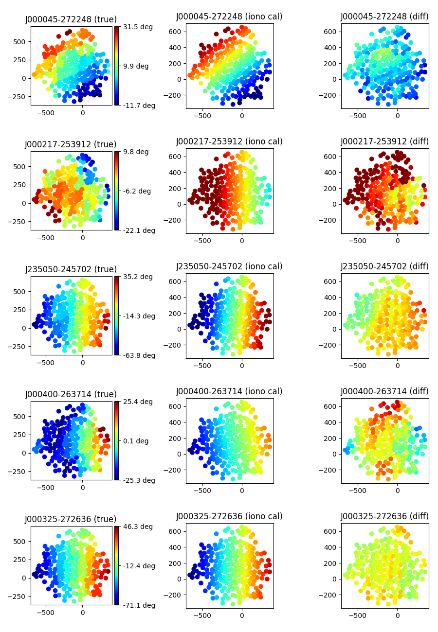
Some examples of the structure across the SKA1-LOW core are given below. The five rows show phase-shift snapshots across the core for five directions. The left column shows the true phase shifts, the middle shows the Cddcalibrator solutions, and the right column shows the difference. The linear approximation is reasonable, but not perfect.

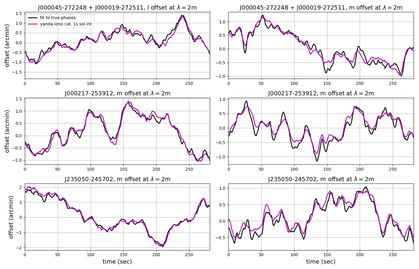
To compare these data further, a similar fit can be applied to the true phase shifts, e.g.:

for t in range(0,Ntime):
    for it in range(0,10):
        A = matrix(zeros((len(stations),2)))
        r = matrix(zeros((len(stations),1)))
        for pix in range(0,len(pixels)):
            for stn in range(0,len(stations)):
                # only mult by wl, since u and v are still in metres
                model = -2.*pi * wl[chan] * ( u[stations[stn]]*alphal[pix,t] + v[stations[stn]]*alpham[pix,t] )

                A[stn,0] += -2.*pi * wl[chan] * u[stations[stn]]
                A[stn,1] += -2.*pi * wl[chan] * v[stations[stn]]
                r[stn,0] += data[pix,stn,t] - model

            sol = (A.T*A).I * A.T*r
            alphal[pix,t] += sol[0,0]
            alpham[pix,t] += sol[1,0]

These can be plotting along with the Cddcalibrator solutions:

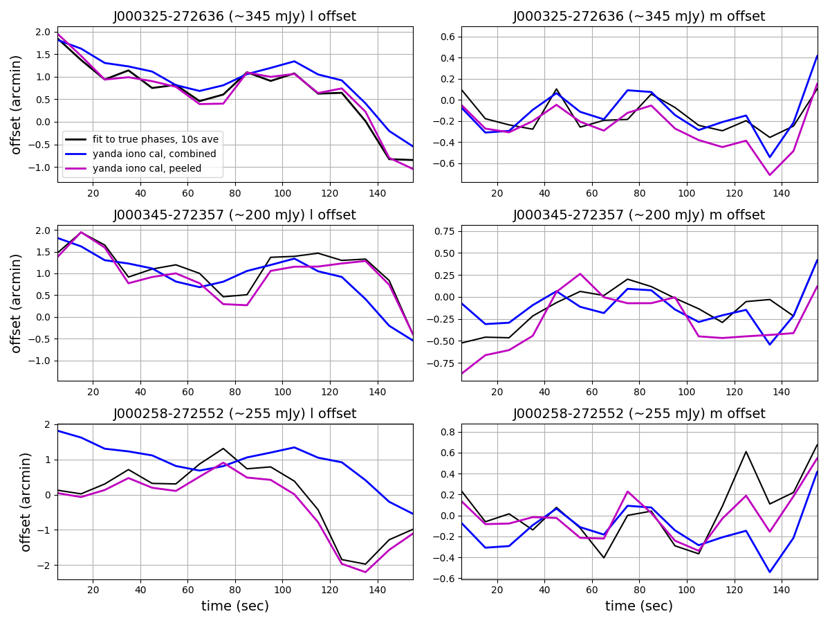
When sources are weaker and closer together, either joint or simultaneous calibration may be needed. Consider the four radio sources indicated in the figure below.

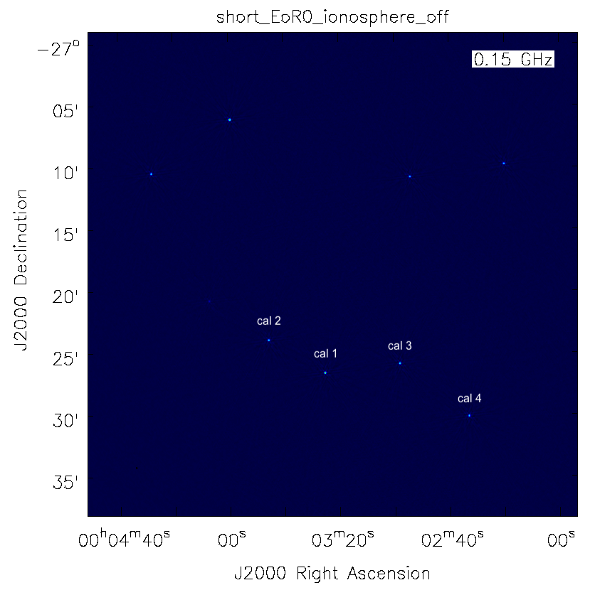
Calibrating towards these sources as separate calibrators can be achieved using:

Cddcalibrator.sources.names                        = [cal1,cal2,cal3,cal4]

Cddcalibrator.sources.cal1.direction               = [00h00m00.000, -27.00deg, J2000]
Cddcalibrator.sources.cal1.components              = [J000325-272636]
Cddcalibrator.sources.cal2.direction               = [00h00m00.000, -27.00deg, J2000]
Cddcalibrator.sources.cal2.components              = [J000345-272357]
Cddcalibrator.sources.cal3.direction               = [00h00m00.000, -27.00deg, J2000]
Cddcalibrator.sources.cal3.components              = [J000258-272552]
Cddcalibrator.sources.cal4.direction               = [00h00m00.000, -27.00deg, J2000]
Cddcalibrator.sources.cal4.components              = [J000232-273008]
Cddcalibrator.sources.J000325-272636.flux.i        = 0.69
Cddcalibrator.sources.J000325-272636.direction.ra  = +0.013252
Cddcalibrator.sources.J000325-272636.direction.dec = -0.007787
Cddcalibrator.sources.J000345-272357.flux.i        = 0.40
Cddcalibrator.sources.J000345-272357.direction.ra  = +0.014577
Cddcalibrator.sources.J000345-272357.direction.dec = -0.007024
Cddcalibrator.sources.J000258-272552.flux.i        = 0.51
Cddcalibrator.sources.J000258-272552.direction.ra  = +0.011494
Cddcalibrator.sources.J000258-272552.direction.dec = -0.007562
Cddcalibrator.sources.J000232-273008.flux.i        = 0.36
Cddcalibrator.sources.J000232-273008.direction.ra  = +0.009866
Cddcalibrator.sources.J000232-273008.direction.dec = -0.008794

Cddcalibrator.nCal                                 = 4

While calibrating against a combined sky model can be achieved using:

Cddcalibrator.sources.names                        = [cal1]

Cddcalibrator.sources.cal1.direction               = [00h00m00.000, -27.00deg, J2000]
Cddcalibrator.sources.cal1.components              = [J000325-272636,J000345-272357,J000258-272552,J000232-273008]
Cddcalibrator.sources.J000325-272636.flux.i        = 0.69
Cddcalibrator.sources.J000325-272636.direction.ra  = +0.013252
Cddcalibrator.sources.J000325-272636.direction.dec = -0.007787
Cddcalibrator.sources.J000345-272357.flux.i        = 0.40
Cddcalibrator.sources.J000345-272357.direction.ra  = +0.014577
Cddcalibrator.sources.J000345-272357.direction.dec = -0.007024
Cddcalibrator.sources.J000258-272552.flux.i        = 0.51
Cddcalibrator.sources.J000258-272552.direction.ra  = +0.011494
Cddcalibrator.sources.J000258-272552.direction.dec = -0.007562
Cddcalibrator.sources.J000232-273008.flux.i        = 0.36
Cddcalibrator.sources.J000232-273008.direction.ra  = +0.009866
Cddcalibrator.sources.J000232-273008.direction.dec = -0.008794

Cddcalibrator.nCal                                 = 1

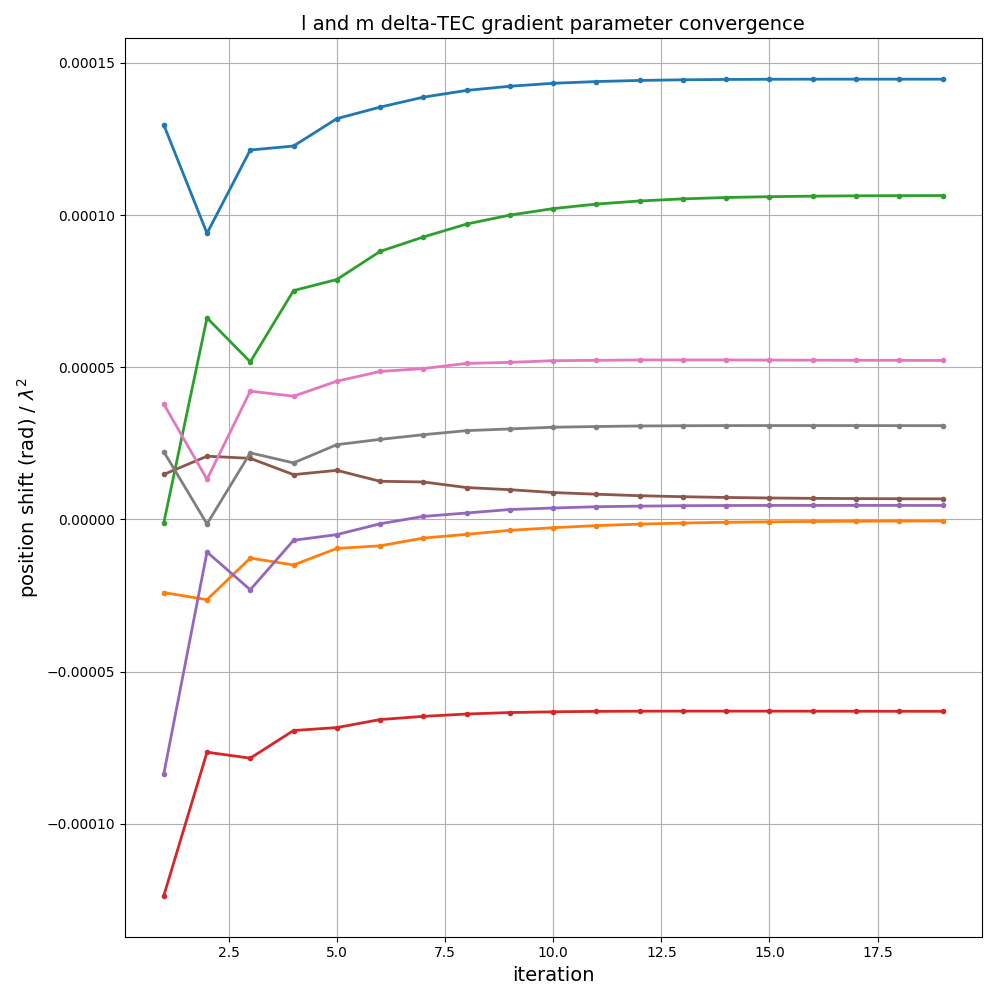
The solutions for these two approaches is shown below for three of these sources, followed by a plot of solution convergence for the first time step.