Basic Continuum Imaging Tutorial
This tutorial demonstrates basic continuum imaging using ASKAPsoft, with a simulated observation that aims to replicate a “typical” observation with BETA. This tutorial will cover the following tasks:
Download of the measurement sets
Calibration of individual beams using observations of 1934-638
Imaging of a simulated science observation of a complex continuum sky, including application of the gains calibration
Mosaicking individual beam images to form a full-field continuum image
Observation summary
The data to be reduced consists of two distinct parts.
The first has 9 short (6 minute) simulated observations of 1934-638, one for each of the 9 beams. Each observation has its own measurement set. These used the BETA array, covering 304 MHz at full spectral resolution (16416 channels), between 746 and 1050 MHz. Thermal noise (Tsys=50K), plus a single set of random gains, have been added to the visibilities. Summary of the specifications:
Target: 1934-638
Direction: RA=19:39:25.036, Dec=-63:42:45.63 (J2000)
Observation length: 6 minutes per beam
Integration time: 5 seconds
Number of beams: 9 per observation
Polarisations: XX & YY
Number of spectral channels: 16416
Channel width: 18.518518 kHz
Tsys: 50K
Gains corruption: Yes
The second is a long (12 hour) simulated observation of a “science field”. The sky model used in the field is our standard “SKADS” field, which uses continuum sources from the SKADS S3-SEX simulation (Wilman et al (2008), MNRAS 388, 1385). Each component has its own spectral index, which should be recoverable from the imaging results. The observation had the same spectral backend as the calibration observations, as well as thermal noise and gains corruption (using the same random gains as the calibration observations).
Summary of the specifications:
Target: SKADS field
Direction: RA=12:30:00.00, Dec=-45:00:00.0 (J2000)
Observation length: 12 hours
Integration time: 5 seconds
Number of beams: 9
Polarisations: XX & YY
Number of spectral channels: 16416
Channel width: 18.518518 kHz
Tsys: 50K
Gains corruption: Yes
Prerequisites
You should read the Central Processor Platform documentation and in particular have setup your environment per the section entitled “Setting up your account”.
You should also have read the Platform Introduction Tutorial and be comfortable with submitting jobs and monitoring their status.
Setting up a working directory
Your working directory will not be within your home directory, instead it will reside on the fast Lustre filesystem:
cd /scratch2/askap/$USER
mkdir continuumtutorial
cd continuumtutorial
lfs setstripe -c 4 .
The lfs setstripe command configures a Lustre file system attribute for this directory. It tells Lustre to stripe files accross 4 storage nodes, for performance reasons.
Retrieving the tutorial dataset
There are 10 measurement sets associated with this tutorial. There are nine for the calibration observations (one per beam), named calibrator_J1934m638_forSKADS_BEAM0.ms through calibrator_J1934m638_forSKADS_BEAM8.ms (these are 2.6GB each). The science field has one measurement set, at full spectral resolution, named sciencefield_SKADS.ms (290.1GB), along with an averaged version of this (channels averaged to 1MHz), named sciencefield_SKADS_coarse.ms (8.1GB).
The datasets for this observation are located on the /group filesystem, and you can copy them to your local directory:
> cp -r /group/askap/askapops/tutorials/BasicContinuum .
> ls BasicContinuum
calibrator_J1934m638_forSKADS_BEAM0.ms  calibrator_J1934m638_forSKADS_BEAM3.ms  calibrator_J1934m638_forSKADS_BEAM6.ms  sciencefield_SKADS_coarseChan.ms
calibrator_J1934m638_forSKADS_BEAM1.ms  calibrator_J1934m638_forSKADS_BEAM4.ms  calibrator_J1934m638_forSKADS_BEAM7.ms  sciencefield_SKADS.ms
calibrator_J1934m638_forSKADS_BEAM2.ms  calibrator_J1934m638_forSKADS_BEAM5.ms  calibrator_J1934m638_forSKADS_BEAM8.ms
Calibration
The first step is to use the ccalibrator program to solve the gains calibration. This will be done using the calibrator observations, and will be applied to the science observation.
Here is a basic parameter set for use with ccalibrator. It has the same sort of structure as the imaging one you would have seen in the intro tutorial, with a few calibration-specific parameters. As usual, refer to the documentation pages on calibration, gridding and so forth for more details.:
Ccalibrator.dataset                         = BasicContinuum/calibrator_J1934m638_forSKADS_BEAM0.ms
Ccalibrator.nAnt                            = 6
Ccalibrator.nBeam                           = 9
Ccalibrator.solve                           = gains
#
Ccalibrator.calibaccess                     = parset
Ccalibrator.calibaccess.parset              = caldata-BEAM0.dat
#
Ccalibrator.sources.names                   = [field1]
Ccalibrator.sources.field1.direction        = [19h39m25.036, -63.42.45.63, J2000]
Ccalibrator.sources.field1.components       = src
Ccalibrator.sources.src.calibrator          = 1934-638
#
Ccalibrator.gridder                         = SphFunc
#
Ccalibrator.ncycles                         = 5
This parset will solve for the gains for the first calibrator observation. We only care about the BEAM 0 from this observation (which is the beam pointing at 1934), but the task actually tries to solve for all beams.
The calibration is done assuming a model of 1934-638 (the Ccalibrator.sources.src.calibrator=1934-638 entry); this is a special unresolved component that accounts for 1934’s spectral variation. It puts the component at the position indicated, which happens to be the direction of the observation. Note the particular format of the direction string, especially the declination!
Save the above parset into a file named calibrator-BEAM0.in. To run this, we need to create an sbatch file, say, calibrator-BEAM0.sbatch:
#!/bin/bash -l
#SBATCH --time=01:00:00
#SBATCH --ntasks=1
#SBATCH --ntasks-per-node=1
#SBATCH --job-name=ccal0
#SBATCH --export=NONE

aprun -n 1 -N 1 ccalibrator -c calibrator-BEAM0.in > calibrator-BEAM0_${SLURM_JOB_ID}.log
This runs as a serial job, and can be submitted in the usual fashion via:
sbatch calibrator-BEAM0.sbatch
Gains Parameters
The gains parameters, one for each polarisation, antenna and beam, are written to a file caldata-BEAM0.dat. This has entries that look like the following:
gain.g11.0.0 = [0.27819,0.680617]
gain.g11.0.1 = [1.10205,0.0753065]
gain.g11.0.2 = [0.554685,-0.540324]
gain.g11.0.3 = [0.670682,0.959503]
gain.g11.0.4 = [1.14376,-0.171543]
gain.g11.0.5 = [1.14408,-0.0398638]
gain.g11.0.6 = [-0.737403,0.560088]
gain.g11.0.7 = [1.02336,-0.255945]
gain.g11.0.8 = [-0.818433,-0.248333]
gain.g11.1.0 = [-0.631561,-0.409769]
gain.g11.1.1 = [1.29398,0.052276]
gain.g11.1.2 = [0.547655,0.834172]
gain.g11.1.3 = [0.271391,-0.790379]
gain.g11.1.4 = [0.380629,0.674252]
gain.g11.1.5 = [0.629311,0.410911]
gain.g11.1.6 = [-0.0787903,1.00496]
gain.g11.1.7 = [0.41577,-0.881319]
gain.g11.1.8 = [0.569721,-0.565723]
This file is just a parset, with each line being a parameter specification. Its format is described in more detail in Access to calibrator solutions, but the format is basically gain.pol.antenna.beam. The only relevant entries from this calibration job are those for beam 0 - that is, those with the gain parameter name ending in .0.
Gains for each beam
The above finds the correct gains for beam 0. To solve them for all other beams, we need to do the same for beams 1-8. To do this for beam 1, we copy the parset to calibrator-BEAM1.in and change “BEAM0” in the dataset name to “BEAM1”. Similarly, copy the sbatch file to calibrator-BEAM1.sbatch and replace “BEAM0” in the filenames with “BEAM1”, then submit.
All other parameters (for now) can remain the same. The direction, importantly, is the same as this is the phase centre for the observation, which has been defined such that it is in the centre of the beam of interest for each measurement set.
This is something that could easily be scripted in one of a variety of ways - this is left as an exercise for the reader! By the end, you should have a set of calibration parsets caldata-BEAM0.dat through caldata-BEAM8.dat. These will be used to calibrate the individual beam images that will be made next.
Note that something you can not do is run this as an MPI job trying to get each processor to process a separate beam – ccalibrator does not work this way. The bandpass calibrator cbpcalibrator has more flexibility in distributed processing, but we don’t need it here as the simulated data has no bandpass structure in the corruption.
Channel averaging
The first step in imaging is to average the visibilities to 304 1MHz channels. There is a measurement set provided that has already had this done, but in case you want to do it yourself, here are the instructions. The averaging is done with the mssplit command (read mssplit (Measurement Splitting/Averaging Utility) for further information) - here is a typical parset:
# Input measurement set
# Default: <no default>
vis         = BasicContinuum/sciencefield_SKADS.ms

# Output measurement set
# Default: <no default>
outputvis   = my_sciencefield_SKADS_coarse.ms

# The channel range to split out into its own measurement set
# Can be either a single integer (e.g. 1) or a range (e.g. 1-300). The range
# is inclusive of both the start and end, indexing is one-based.
# Default: <no default>
channel     = 1-16416

# Defines the number of channel to average to form the one output channel
# Default: 1
width       = 54
Note that the output MS has a slightly different filename to the averaged MS provided, and is not in the BasicContinuum directory.
Save this parset into a file named mssplit.in. To run this, we need to create a sbatch file, say, mssplit.sbatch:
#!/bin/bash -l
#SBATCH --time=04:00:00
#SBATCH --ntasks=1
#SBATCH --ntasks-per-node=1
#SBATCH --job-name=mssplit
#SBATCH --export=NONE

aprun -n 1 -N 1 mssplit -c mssplit.in > mssplit_${SLURM_JOB_ID}.log
This runs as a serial job, using only a single processor. Run this in the usual fashion via:
sbatch mssplit.sbatch
Make a note of the ID that sbatch returns - you may need this to set up dependencies later on (see the imaging section below).
Imaging
To do the imaging we select individual beams and image them independently. This is to replicate what is necessary for actual BETA data as the phase/delay tracking is done independently for each antenna, and this, combined with the poor knowledge of the primary beam, means the joint deconvolution (ie. of all beams at once) will not be reliable.
The imaging is done similarly to that in the introductory tutorial, with two additions. One, we will select an individual beam from the measurement set, and two, we will add some cleaning. Here is an example parset:
Cimager.dataset                                 = BasicContinuum/sciencefield_SKADS_coarse.ms
Cimager.Feed                                    = 0
#
# Each worker will read a single channel selection
Cimager.Channels                                = [1, %w]
#
Cimager.Images.Names                            = [image.i.clean.sciencefield.BEAM0]
Cimager.Images.shape                            = [2048,2048]
Cimager.Images.cellsize                         = [10arcsec,10arcsec]
Cimager.Images.image.i.clean.sciencefield.BEAM0.frequency   = [898.e6, 898.e6]
Cimager.Images.image.i.clean.sciencefield.BEAM0.nchan       = 1
Cimager.Images.image.i.clean.sciencefield.BEAM0.direction   = [12h30m00.00, -45.00.00.00, J2000]
Cimager.Images.image.i.clean.sciencefield.BEAM0.nterms      = 2
#
# The following are needed for MFS clean
# This one assigns one worker for each of the 3 Taylor terms
Cimager.nworkergroups                           = 3
# This tells the gridder to weight the visibilities appropriately
Cimager.visweights                              = MFS
# This is the reference frequency - it should lie in your frequency range (ideally in the middle)
Cimager.visweights.MFS.reffreq                  = 898.e6
#
# This defines the parameters for the gridding.
Cimager.gridder.snapshotimaging                 = true
Cimager.gridder.snapshotimaging.wtolerance      = 2600
Cimager.gridder                                 = WProject
Cimager.gridder.WProject.wmax                   = 2600
Cimager.gridder.WProject.nwplanes               = 99
Cimager.gridder.WProject.oversample             = 4
Cimager.gridder.WProject.diameter               = 12m
Cimager.gridder.WProject.blockage               = 2m
Cimager.gridder.WProject.maxfeeds               = 9
Cimager.gridder.WProject.maxsupport             = 512
Cimager.gridder.WProject.variablesupport        = true
Cimager.gridder.WProject.offsetsupport          = true
Cimager.gridder.WProject.frequencydependent     = true
#
# This defines the cleaning/deconvolution setup
Cimager.solver                                  = Clean
Cimager.solver.Clean.algorithm                  = BasisfunctionMFS
Cimager.solver.Clean.niter                      = 5000
Cimager.solver.Clean.gain                       = 0.5
Cimager.solver.Clean.scales                     = [0, 3, 10]
Cimager.solver.Clean.verbose                    = False
Cimager.solver.Clean.tolerance                  = 0.01
Cimager.solver.Clean.weightcutoff               = zero
Cimager.solver.Clean.weightcutoff.clean         = false
Cimager.solver.Clean.psfwidth                   = 512
Cimager.solver.Clean.logevery                   = 100
Cimager.threshold.minorcycle                    = [30%, 0.9mJy]
Cimager.threshold.majorcycle                    = 1mJy
Cimager.ncycles                                 = 4
Cimager.Images.writeAtMajorCycle                = false
#
# This section is for the preconditioning (weighting)
Cimager.preconditioner.Names                    = [Wiener, GaussianTaper]
Cimager.preconditioner.GaussianTaper            = [30arcsec, 30arcsec, 0deg]
Cimager.preconditioner.Wiener.robustness        = 0.0
Cimager.preconditioner.Wiener.taper             = 64
#
# Whether to restore the final image and what beam to use
Cimager.restore                                 = true
Cimager.restore.beam                            = fit
#
# Apply calibration, and from where
Cimager.calibrate                               = true
Cimager.calibaccess                             = parset
Cimager.calibaccess.parset                      = caldata-BEAM0.dat
Cimager.calibrate.scalenoise                    = true
Cimager.calibrate.allowflag                     = true
Save the above parameter set in a file named clean-BEAM0.in. Before running this, let’s look at a few key features of this parset. First is this:
Cimager.Feed = 0
This does the selection-by-beam, where we only use data for feed=0 in the measurement set. Note that the above example uses the averaged measurement set provided in the tarball you downloaded. If you ran the averaging with mssplit yourself you can change the MS name to match.
The calibration is applied by the following:
Cimager.calibrate                           = true
Cimager.calibaccess                         = parset
Cimager.calibaccess.parset                  = caldata-BEAM0.dat
Cimager.calibrate.scalenoise                = true
Cimager.calibrate.allowflag                 = true
where we choose the calibration parameters parset that was produced by ccalibrator for the beam we are selecting.
We grid the data using the WProject gridder. We choose this for this simulation, since it does not include any primary beam correction. We don’t know the primary beam for BETA well enough, so we grid with WProject, then apply analytic primary beam weights in the mosiacking stage.
We are doing multi-frequency synthesis for this image. This is controlled by the following parameters:
Cimager.visweights                          = MFS
Cimager.visweights.MFS.reffreq              = 898.e6
This will result in the creation of “Taylor-term images”. These represent the Taylor terms that represent the frequency dependence of each spatial pixel. The different terms relate to the spectral index (alpha) and spectral curvature (beta) of the spectrum, which can be defined through a second-order polynomial in log-space, shown in the first two equations below. The third equation shows the result of a Taylor expansion about the reference frequency.

The Taylor term images then contain the coefficients of this expansion, so that the image with suffix .taylor.0 contains I(nu0), .taylor.1 contains I(nu0)*alpha, and .taylor.2 contains I(nu0)*(0.5*alpha*(alpha-1)+beta). The reference frequency is given by the Cimager.visweights.MFS.reffreq parameter (in Hz) - this should be in the middle of the band for optimal performance.
The cleaning is controlled by these parameters:
Cimager.solver                              = Clean
Cimager.solver.Clean.algorithm              = BasisfunctionMFS
and those following. The algorithm BasisfunctionMFS is a good way of doing the multi-scale multi-frequency synthesis. Read Solvers for information on all the clean options. The multi-scale part is controlled by:
Cimager.solver.Clean.scales = [0, 3, 10]
This will clean with components of size 0 pixels (ie. point sources), 3 pixels and 10 pixels.
Finally, note that the above parset has:
Cimager.Images.writeAtMajorCycle = false
Setting this to true can be useful if you want to look at the intermediate major cycles of the cleaning, but it does produce a lot more images. To save clutter we’ll keep it at false for now.
To run the imaging, we need an sbatch file - call it clean-BEAM0.sbatch:
#!/bin/bash -l
#SBATCH --time=03:00:00
#SBATCH --ntasks=913
#SBATCH --ntasks-per-node=20
#SBATCH --job-name=clean0
#SBATCH --export=NONE

aprun -n 913 -N 20 cimager -c clean-BEAM0.in > clean-BEAM0_${SLURM_JOB_ID}.log
Note that the number of processes has increased compared to the intro tutorial. That’s because we are doing MFS imaging, and we have requested:
Cimager.nworkergroups = 3
in the parset. This assigns each Taylor term to a separate processor, to spread the work and help speed things up. This way, we now have (3 worker groups * 304 channels + 1 master) processes (i.e. 913).
You can submit this in the usual way, but if you have run the mssplit job, this may still be going, and it needs that to finish first. You can still submit the imaging job, but make it depend on the successful completion of the mssplit job. If the ID of the mssplit job is 1234, then you can submit the imaging job via:
sbatch -d afterok:1234 clean-BEAM0.sbatch
Once this completes, you will have a larger set of image products than was produced for the dirty imaging in the intro tutorial:
Filename |
Description |
|---|---|
image.i.clean.sciencefield.BEAM0 |
The clean model image - pixel map of the clean components. |
image.i.clean.sciencefield.BEAM0.restored |
The cleaned, restored image. |
mask.i.clean.sciencefield.BEAM0 |
The normalised mask showing the scaling of sensitivity due to the primary beam. |
psf.i.clean.sciencefield.BEAM0 |
The natural PSF image (transform of the UV coverage). |
psf.image.i.clean.sciencefield.BEAM0 |
The PSF image after preconditioning (weighting, tapering). This is the actual PSF of the image |
residual.i.clean.sciencefield.BEAM0 |
Residual image |
sensitivity.i.clean.sciencefield.BEAM0 |
Sensitivity pattern image |
weights.i.clean.sciencefield.BEAM0 |
Weights image |
The restored image should look something like the following (for the BEAM0 case).
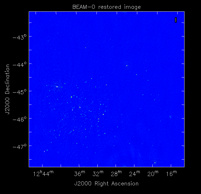
The image size has been chosen so that it is sufficient for the full mosaic image, and has the phase centre of the observation at the middle, but the portion imaged only includes our selected beam. Since we have used the WProject gridder, the weights image will be flat (the AWProject gridder produces weights images showing the primary beam pattern, but we are avoiding this for early BETA imaging).
However, it also means that the fluxes of sources in these individual beam images will be increasingly incorrect as we move away from the beam centre. For instance, the bright source near RA=12:26, Dec=-44, is actually >3Jy, but we measure its flux in BEAM0 as only about 62mJy. We will correct for this in the mosaicking step below.
Mosaicking
We repeat the imaging for each beam, imaging only a single beam each time, so that we get images for BEAM0 through BEAM8. Once this is done, we need to mosaic the images together to form the final full-field image. This is done with the linmos program, information on which can be found at linmos (Linear Mosaic Applicator).
The mosaicking program is driven by a simple parameter set. Consider the following:
linmos.names            = [BEAM0..8]
linmos.findmosaics      = true
linmos.weighttype       = FromPrimaryBeamModel
linmos.weightstate      = Inherent
linmos.feeds.centre     = [12h30m00.00, -45.00.00.00]
linmos.feeds.spacing    = 1deg
linmos.feeds.BEAM0      = [-1.0, -1.0]
linmos.feeds.BEAM1      = [-1.0,  0.0]
linmos.feeds.BEAM2      = [-1.0,  1.0]
linmos.feeds.BEAM3      = [ 0.0, -1.0]
linmos.feeds.BEAM4      = [ 0.0,  0.0]
linmos.feeds.BEAM5      = [ 0.0,  1.0]
linmos.feeds.BEAM6      = [ 1.0, -1.0]
linmos.feeds.BEAM7      = [ 1.0,  0.0]
linmos.feeds.BEAM8      = [ 1.0,  1.0]
linmos.psfref           = 4
linmos.nterms           = 2
This aims (via the findmosaics=true parameter) to do the mosaicking for all sets of images that fit the pattern given in the names parameter. The double-fullstop indicates a range of numbers to iterate over. The output name, which isn’t given in findmosaics mode, is instead determined by replacing the pattern in the names parameter with linmos.
All sets of images that fit the pattern will be mosaicked. This will include, in our example, model & restored images for each taylor term, as well as residual, sensitivity and weights images.
The weights are determined here by providing primary beam models, as well as a list of locations of these beams - one for each input image. These primary beam models are simple circularly-symmetric Gaussian functions, with FWHM determined from the frequency of the image being mosaicked. By giving weightstate = Inherent, we assume that the input image reflects the primary beam response (which it does when imaged with the WProject gridder), and the mosaicking corrects for this so that the fluxes of sources are correct across the field.
The psfref parameter indicates from which number out of that sequence the restoring beam information should be taken. This is necessary as the restoring beam could be different for different images (due to the effect of different calibration).
The nterms parameter tells linmos to look for taylor term images, and make multiple output images, one for each taylor term present.
Save this parset into a file, say linmos_image.in, and then create an sbatch file as before, say, linmos_image.sbatch:
#!/bin/bash -l
#SBATCH --time=01:00:00
#SBATCH --ntasks=1
#SBATCH --ntasks-per-node=1
#SBATCH --job-name=linmos
#SBATCH --export=NONE

aprun -n 1 -N 1 linmos -c linmos_image.in > linmos_image_${SLURM_JOB_ID}.log
(again, this is using only a single processor, as linmos is a serial application) and run via:
sbatch linmos_image.sbatch
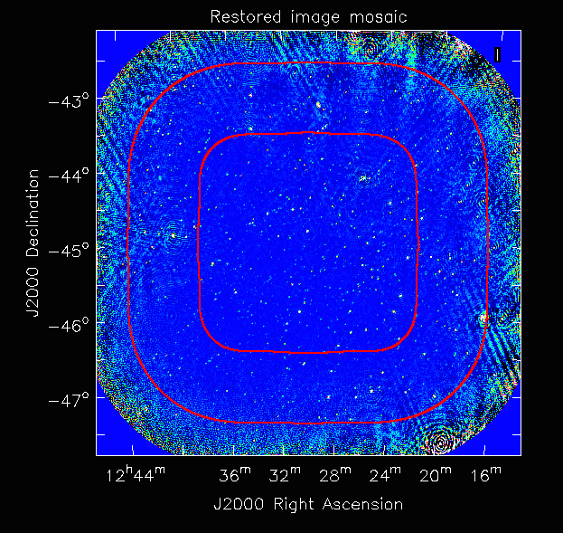
This job will produce model, restored, weights, residual and sensitivity images for each of the taylor terms. See Platform Introduction Tutorial for details on visualisation of your images. The full mosaicked restored image (image.i.clean.sciencefield.linmos.taylor.0.restored) should look something like the following image. The red lines indicate the weights contours for 50% (inner line) and 1% (outer line) of the peak weight. Note that the outer edges of the field now have increased noise due to the scaling-up of the low-weight points (by the weighttype=Inherent correction).
Exploring the imaging parameters
Close examination of the resulting image will show various features and artefacts that one might want to address. There are noticeable sidelobes near some of the brighter sources in the top and top-right, for instance, as well as radial features near the bright source to the left. Some examples of alternative tests to try:
Does it just require deeper cleaning? You can change the number of major cycles using the Cimager.ncycles parameter (you may need to increase the time requested in the sbatch file.) You can also change the threshold levels for both the minor and major cycles (Cimager.threshold.minorcycle and Cimager.threshold.majorcycle).
Is the multi-scale clean capturing all the necessary structure? (This may be important for the bright, extended source at top.) You could try adding a larger-scale term to the Cimager.solver.Clean.scales list, although this can result in large-scale noise being added as well, so beware (I have tried it with [0,3,10,30], and found large scale ripples appeared - perhaps these would disappear with better weighting. See the next point).
The preconditioning of the data will likely have an effect as well. The imaging done above used both Wiener filtering and Gaussian tapering, and both of these can be altered or removed. Some idea of the effect of different values of the parameters can be seen on Emil’s PSF simulations page (which I’ve moved to my website, but it remains the same…).
The fidelity of the image can also be improved by tweaking the gridding parameters, although this can be fiddly. Increasing the oversampling, for instance, can improve the image quality at the expense of greater memory usage. If your job fails due to running out of memory, you can decrease the number of processors per node - change the ntasks-per-node to 16, say, from 20, as well as the -N flag for the aprun call. You will likely have to increase the maxsupport parameter as well - try going up in factors of 2. See Gridders for explanations of the gridding parameters.