Selavy Source-Finding Tutorial
This tutorial demonstrates the use of the Selavy sourcefinder to find sources in an image, and fit components to them. This will take the image produced from the Basic Continuum Imaging Tutorial tutorial and demonstrate different approaches to building up a source catalogue.
The various options of Selavy are described in detail in the Source-Finding Documentation section, and this tutorial will not attempt to demonstrate all possible modes. We will focus primarily on the needs of continuum imaging.
Prerequisites
This tutorial uses the outputs from the imaging tutorial, specifically the restored Taylor term images and, optionally, the weights images. However, the scripts can be used with essentially any image: Selavy is able to read both CASA and FITS format. To find the spectral index & curvature of sources, you will need Taylor term images - these are found automatically if the input image is named in the same way as the output from cimager, but you can directly specify them (see Post-processing of detections for details).
A simple search
The first demonstration will be a simple search to a given flux threshold, in this case 100mJy. Sources that lie above this threshold are “grown” to a secondary threshold of 50mJy, and then have Gaussian components fitted to them.
Pixels that lie above the primary threshold are identified and grouped together into ‘islands’. These are then grown out to include all neighbouring pixels above the secondary threshold - pixels with fluxes between these two thresholds are only included if they are attached to pixels above the primary threshold.
When fitting is requested, Gaussian components are fitted to the islands and their parameters written to a separate catalogue. It is typically this catalogue that one would use in analysing continuum observations, or, for instance to construct a sky model.
Here is the parset used for this search:
# The image to be searched
Selavy.image = image.i.clean.sciencefield.linmos.taylor.0.restored
#
# We will search just a subsection of the image
Selavy.flagSubsection = true
# The subsection shows the pixel range for each axis, giving the
#  first & last pixel to be used (1-based).
Selavy.subsection = [251:1800,251:1800,*,*]
#
# This is how we divide it up for distributed processing, with the
#  number of subdivisions in each direction, and the size of the
#  overlap region in pixels
Selavy.nsubx = 6
Selavy.nsuby = 3
Selavy.overlapx = 50
Selavy.overlapy = 50
#
# The search threshold, in the flux units of the image
Selavy.threshold = 0.1
# Grow the detections to a secondary threshold
Selavy.flagGrowth = true
Selavy.growthThreshold = 0.05
#
# Parameters to switch on and control the Gaussian fitting
Selavy.Fitter.doFit = true
Selavy.Fitter.fitTypes = [full]
Selavy.Fitter.maxNumGauss = 2
#
# Size criteria for the final list of detected islands
Selavy.minPix = 3
Selavy.minVoxels = 3
Selavy.minChannels = 1
#
# How the islands are sorted in the final catalogue - by
#  integrated flux in this case
Selavy.sortingParam = iflux
If one saves this to a parset file selavy.in, say, then it can be run using the following sbatch file:
#!/bin/bash -l
#SBATCH --time=01:00:00
#SBATCH --ntasks=19
#SBATCH --ntasks-per-node=19
#SBATCH --job-name=selavy

log=selavy-${SLURM_JOB_ID}.log

aprun -N 19 -n 19 selavy -c selavy.in > $log
This example demonstrates several elements of Selavy. First, it is run in distributed mode, where the image is split up so that each worker process only processes a small fraction of the image. The way it is split up is governed by the nsubx and nsuby parameters, being the number of subimages in the x- and y-directions, and the overlap between subimages (in pixels) is controlled by the overlapx and overlapy parameters. The overlap ensures we don’t miss structure at the boundaries.
The fitting is switched on by setting Fitter.doFit = true (it is off by default). There are many options possible in the fitting, which are detailed in Post-processing of detections. The setup in this example limits the fitting to either one or two Gaussian components - one is fit first and is accepted if the fit works and passes chi-squared & RMS tests, else a two component fit is tried. If both fail, the initial estimates are returned.
Outputs
This first example used a relatively high threshold (it’s actually about 70-sigma for the simulated image), and runs very quickly (ie. less that a second), finding 49 sources in the simulated image and fitting Gaussian components to them.
The key output files are as follows:
Filename |
Parameters |
Description |
|---|---|---|
selavy-results.txt |
resultsFile |
The catalogue of detected islands and their parameters. |
selavy-results.xml |
votFile |
A VOTable version of the islands catalogue. |
selavy-results.ann |
karmaFile / flagKarma |
A karma annotation file showing the locations of the islands. |
selavy-results.reg |
ds9File / flagDS9 |
A DS9 region file showing the island locations |
selavy-results.crf |
casaFile / flagCASA |
A CASA region file showing the island locations |
selavy-fitResults.txt |
fitResultsFile |
The catalogue of fitted components. |
selavy-fitResults.xml |
<no specific parameter> |
A VOTable version of the fitted components catalogue. |
selavy-fitResults.{ann,reg,crf} |
fitAnnotationFile |
Annotation/region files showing the location of the fitted components. |
selavy-SubimageLocations.ann |
subimageAnnotationFile |
Karma annotation file showing the borders of the subimages. |
There are two catalogues written: selavy-results.txt is the Duchamp-style catalogue showing the detected islands and their parameters; and selavy-fitResults.txt is the catalogue of fitted components. The ID of the fitted components has a number and one or more letters - the number refers to the ID of the island in selavy-results.txt, while the letters give the order of the component (ordered by flux) within that island. The first 26 will have a single letter a-z, then aa-zz, then aaa-zzz and so forth.
The .txt files are simple formatted ASCII tables. They have XML/VOTable equivalents written as well - these are standard VOTable format that can be used in applications such as TOPCAT and Aladin.
There are annotation and region files produced that allow the detected sources to be displayed in either kvis (the .ann files), DS9 (the .reg files) or casaviewer (either .reg or .crf are possible). These will show the outline of the detected island, or ellipses indicating the fitted components. There is also a karma annotation file showing the locations of the worker subimages.
The catalogue of islands is the same as the results file produced by Duchamp, and has the following format. It starts with a listing of the parameters (this is what is produced by the Duchamp code, so Selavy-specific parameters are not typically reproduced here) and a summary of the thresholds and number of detections. All these lines are started with a # character. Then there is the actual catalogue, in ASCII format:
# Results of the Duchamp source finder v.1.6.1: Wed Jun  4 09:53:19 2014
#
# ---- Parameters ----
# Image to be analysed.............................[imageFile]  =  image.i.clean.sciencefield.linmos.taylor.0.restored[251:1800,251:1800,1:1,1:1]
# Intermediate Logfile...............................[logFile]  =  selavy-Logfile.Master.txt
# Final Results file.................................[outFile]  =  selavy-results.txt
# VOTable file.......................................[votFile]  =  selavy-results.xml
# Karma annotation file............................[karmaFile]  =  selavy-results.ann
# DS9 annotation file................................[ds9File]  =  selavy-results.reg
# CASA annotation file..............................[casaFile]  =  selavy-results.crf
# Saving mask cube?...........................[flagOutputMask]  =  false
# Saving 0th moment to FITS file?........[flagOutputMomentMap]  =  false
# Saving 0th moment mask to FITS file?..[flagOutputMomentMask]  =  false
# Saving baseline values to FITS file?....[flagOutputBaseline]  =  false
# ------
# Type of searching performed.....................[searchType]  =  spatial
# Trimming Blank Pixels?............................[flagTrim]  =  false
# Searching for Negative features?..............[flagNegative]  =  false
# Area of Beam (pixels).......................................  =  29.2281   (beam: 5.86614 x 4.39728 pixels)
# Removing baselines before search?.............[flagBaseline]  =  false
# Smoothing data prior to searching?..............[flagSmooth]  =  false
# Using A Trous reconstruction?...................[flagATrous]  =  false
# Using Robust statistics?...................[flagRobustStats]  =  true
# Using FDR analysis?................................[flagFDR]  =  false
# Detection Threshold..............................[threshold]  =  0.1
# Minimum # Pixels in a detection.....................[minPix]  =  3
# Minimum # Channels in a detection..............[minChannels]  =  1
# Minimum # Voxels in a detection..................[minVoxels]  =  3
# Growing objects after detection?................[flagGrowth]  =  true
# Threshold for growth.......................[growthThreshold]  =  0.05
# Using Adjacent-pixel criterion?...............[flagAdjacent]  =  true
# Max. velocity separation for merging........[threshVelocity]  =  7
# Reject objects before merging?.......[flagRejectBeforeMerge]  =  false
# Merge objects in two stages?...........[flagTwoStageMerging]  =  true
# Method of spectral plotting.................[spectralMethod]  =  peak
# Type of object centre used in results..........[pixelCentre]  =  centroid
# --------------------
#
# --------------------
# Summary of statistics:
# Detection threshold = 0.1 Jy/beam
# Detections grown down to threshold of 0.05 Jy/beam
#
# Not calculating full stats since threshold was provided directly.
# --------------------
# Total number of detections = 49
# --------------------
# ---------------------------------------------------------------------------------------------------------------------------------------------------------------------------------------------------------------------------------------------------------------------------------------------------------------------
#  ObjID           Name      X      Y     Z         RA       DEC         RA        DEC          FREQ      MAJ      MIN     PA     w_RA    w_DEC   w_50   w_20 w_FREQ     F_int     F_tot    F_peak   X1   X2   Y1   Y2  Z1  Z2 Nvoxel Nchan Nspatpix Flag   X_av   Y_av  Z_av X_cent Y_cent Z_cent X_peak Y_peak Z_peak
#                                                                     [deg]      [deg]          [Hz] [arcmin] [arcmin]  [deg] [arcmin] [arcmin]   [Hz]   [Hz]   [Hz]      [Jy] [Jy/beam] [Jy/beam]
# ---------------------------------------------------------------------------------------------------------------------------------------------------------------------------------------------------------------------------------------------------------------------------------------------------------------------
       1 J121503-455738 1957.9  656.6   0.0 12:15:03.8 -45:57:38 183.765738 -45.960668 900000000.000     1.01     0.84  11.78     1.42     1.73  0.000  0.000  0.000     0.332     9.714     0.277 1954 1962  652  661   0   0     73     1       73    - 1957.8  656.6   0.0 1957.9  656.6    0.0   1958    657      0
       2 J121529-464245 1919.0  387.5   0.0 12:15:29.2 -46:42:45 183.871519 -46.712521 900000000.000     0.99     0.82 175.89     0.94     1.38  0.000  0.000  0.000     0.106     3.102     0.129 1917 1922  384  391   0   0     37     1       37    - 1919.1  387.5   0.0 1919.0  387.5    0.0   1919    388      0
The components catalogue selavy-fitResults.txt, looks like this:
#      ID           Name         RA        DEC      X      Y     F_int    F_peak F_int(fit) F_pk(fit)  Maj(fit)  Min(fit) P.A.(fit) Maj(fit_deconv.)   Min(fit_deconv.) P.A.(fit_deconv.)   Alpha    Beta Chisq(fit)  RMS(image)  RMS(fit) Nfree(fit) NDoF(fit) NPix(fit) NPix(obj) Guess?
#      --             --      [deg]      [deg]  [pix]  [pix]      [Jy] [Jy/beam]       [Jy] [Jy/beam]  [arcsec]  [arcsec]     [deg]         [arcsec]           [arcsec]             [deg]      --      --         --   [Jy/beam] [Jy/beam]         --        --        --        --     --
       1a J121503-455738 183.765701 -45.960550 1957.9  656.7     0.332     0.277      0.407     0.275    67.246    56.746     22.81           48.391            5.05654            344.13  -6.721   0.000     30.265     0.00664     0.644          6        66        73        73      0
       2a J121529-464245 183.871722 -46.712437 1919.0  387.6     0.106     0.129      0.175     0.129    68.654    50.859    169.99           41.442           14.41590            321.44  -4.951   0.000      1.704     0.00516     0.215          6        30        37        37      0
Note the simpler structure with just the column names and units at the top. This file should be able to be easily read in python using the astropy.table module. Here is some example code that allows you to interact with it:
#!/usr/bin/env python
import astropy.table as table

# read the catalogue
cat = table.Table.read('selavy-fitResults.txt',format='ascii')
# show the column names
cat.colnames
# access the integrated fluxes of the components directly, storing as a numpy array
fint = cat.columns['F_int(fit)'].data
Simple Signal-to-noise thresholding
A simple change to the above parset can make your search be in signal-to-noise terms. Change
# The search thresholds, in the flux units of the image
Selavy.threshold = 0.1
Selavy.flagGrowth = true
Selavy.growthThreshold = 0.05
to
# The search thresholds, in units of sigma above the mean
Selavy.snrCut = 10
Selavy.flagGrowth = true
Selavy.growthCut = 4
and you will do a search for sources above 10-sigma, that are then grown to the 4-sigma level.
The default approach uses the median and median absolute deviation from the median (MADFM), although the mean and standard deviation can be used by setting Selavy.flagRobustStats=false. The robust statistics take a little longer, due to the partial sorting that is involved, but they are probably more reliable, particularly when there is a lot of signal present.
This approach uses the Duchamp method of applying a single threshold to the entire image. When run in distributed mode, as this will be, each worker finds the mean (or median), sends it to the master process which averages them to find the global mean estimator. This is then distributed to the workers who then find their local standard deviation or MADFM. These are again averaged by the master to provide a global estimator of the standard deviation, and hence the threshold. A more complete description of this process can be found in Whiting & Humphreys (2012), PASA 29, 371.
This will take slightly longer than the first example, due to the additional statistics calculation & communication, and because it finds more sources due to the lower threshold. It will still be quick - my example took about 20 seconds to run, finding 560 sources.
Variable signal-to-noise thresholding
Instead of only using a single global threshold, Selavy allows the use of signal-to-noise thresholds that depend only on the noise local to a given pixel. This allows the actual flux threshold to vary according to the image noise, rising where the sensitivity or background due to sidelobes is high, and falling where the sensitivity is very good.
To make use of this, keep the signal-to-noise threshold parameters as shown above, and add the following:
# Turn on the variable threshold option
Selavy.VariableThreshold = true
# Pixel width of box in which to calculate statistics.
Selavy.VariableThreshold.boxSize = 50
# Name of image of detection threshold to be created
Selavy.VariableThreshold.ThresholdImageName=detThresh.img
# Name of image of noise to be created
Selavy.VariableThreshold.NoiseImageName=noiseMap.img
# Name of image of mean pixel level to be created
Selavy.VariableThreshold.AverageImageName=meanMap.img
# Name of image of signal-to-noise ratio to be created
Selavy.VariableThreshold.SNRimageName=snrMap.img
The key parameters are VariableThreshold and VariableThreshold.boxSize, which turn on the feature and set the size of the box in which the statistics and threshold are calculated. A square box of this width is slid over the image, and each pixel has a threshold calculated from the noise statistics of the pixels within the box centred on it.
Images showing the various statistics can be written - only those given in the parset will be written. All images will be the same size as the input image (regardless of what search subsection you have used).
This method also allows you to more confidently drop the detection threshold from those levels used with the global threshold case above, as you won’t be swamped by spurious signal in high-noise areas.
Again, this works with the distributed processing. The overlaps between subimages will be at least twice the box width, as pixels within a box width of the edge of a worker’s image will not be processed (note this if you have things near the edge of your image that you care about).
The execution time for this mode is a bit longer, as the sliding-box calculations require quite a bit more processing (particularly if the robust statistics are used). Even so, my tests completed in about 1.5 minutes, finding about 800 sources.
Alternative modes
This section will detail a few alternative ways of running Selavy
Finding initial component estimates
A key part of the Gaussian fitting is determining an initial estimate of the parameters. Selavy’s original approach (and currently the default) was to apply a number of “sub-thresholds” in between the detection threshold and the peak, and track the number of separate maxima within the island. There are a range of parameters, detailed on Post-processing of detections, that control the details of this algorithm.
While this approach works well, I’ve recently incorporated the algorithm used in Aegean, which uses a curvature map to locate local maxima. See Hancock et al. (2012), MNRAS 422, 1812 for details on the algorithm. I’m currently doing a detailed comparison of the two approaches, but this mode has been made available.
To make use of this option, add the following to your parset:
# Parameters to switch on curvature map analysis and output the
#  curvature image
Selavy.Fitter.useCurvature = true
Selavy.Fitter.curvatureImage = curvature.img
Forcing a PSF fit
It may be that you want to force the Gaussian fitting to fit only PSF-sized components, rather than allowing the size of the components to expand.
To do this, you can choose an alternative mode for the fitting by putting this in your parset:
# This forces the fits to just use PSF-sized components
Selavy.Fitter.fitTypes = [psf]
This will then just fit to the location and flux of the component, keeping the size fixed to that of the beam (as specified in the image header).
You can specify more than one fitting mode, by doing something like:
# This does both a full-parameter fit and a PSF-sized fit
Selavy.Fitter.fitTypes = [full,psf]
This way, point sources will typically be fit by a PSF-sized component, but extended sources will still be fit by a larger Gaussian.
The best fit of the two is chosen on the basis of the reduced chi-squared value from the fit. [Note the discussion in Post-processing of detections about the suitability of the chi-squared value in the case of correlated pixels.]
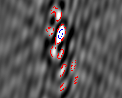
Dealing with bright sidelobes
It may be that you want to extract a component fitting a source with bright sidelobes, for instance from a poorly-cleaned BETA image. Here’s a good procedure for Selavy:
# Fitting parameters, as before
Selavy.Fitter.doFit = true
Selavy.Fitter.fitTypes = [full]
# Limit the number of Gaussians to 1
Selavy.Fitter.maxNumGauss = 1
# Do not use the number of initial estimates to determine how many
#  Gaussians to fit
Selavy.Fitter.numGaussFromGuess = false
# The fit may be a bit poor, so increase the reduced-chisq threshold
Selavy.Fitter.maxReducedChisq = 10.
#
# Allow islands that are slightly separated to be considered a
# single 'source'
Selavy.flagAdjacent = false
# The separation in pixels for islands to be considered 'joined'
Selavy.threshSpatial = 7
This forces a fit of a single Gaussian only (ignoring the full set of initial estimates), and (as of change set 6455, or release CP-0.3) returns the first estimate if the fit fails. Note that the max reduced chisq has been upped to 10 to capture poor fits (often a good idea for bright targets, as the PSF is slightly different to a Gaussian).
Here’s an example, where all the red contours are a single Duchamp source and the blue ellipse represents the fitted component. Some tweaking of the threshSpatial parameter might be needed, depending on the typical separation of the sidelobes