RVS Standalone Client
User Guide
Table Of Contents
Introduction
What is RVS?
What is RVSViewer?
Installation
Running RVSViewer
User Interface
Display Canvas
Image Detail Panel
Position Information Panel
Status Bar
Functions
View Remote Image
Delete Image
Clear Canvas/ Delete multiple images
Position Tracking
Zooming
Change Colormap
Changing Channels in a Cube
Change Imape Options
Options available for all image types
Raster Options
Contour Options
Introduction
What is RVS?
The Remote Visualisation System is a software system that allows remote clients to visualise astronomical data. It is a server-side system, where all the processing is done on the server when requested by a client.
What is the RVSViewer?
RVSViewer is Java application that allows users to visualise FITS images by using the RVS Server. The application takes URL to FITS images and displays the image for the user to analyse. Users may zoom in and out of the image, change the colormap, select specific channels in a cube to view, enable/disable axis labels and change other options of images. The client also allows contours to be overlaid on top of raster images.
Installation
Being a Java implementation, the client executes on all java enabled platforms including Solaris, Linux and Microsoft Windows. There is no installation process for the application besides placing the client jar file somewhere on the file system accessible by the user.
The following are the minimum hardware and software requirements for the client:
- Java enabled platform
- 128MB RAM
- JRE version 1.3.1 or higher
- Java Web Start version 1.1 or higher (For running over the web)
Running the Client
Command Line
The client can be executed by typing the following on the command line:
java -jar rvsviewer.jarwhere rvsviewer.jar is the name of the client jar file.
You may also send width, height and image parameters the application. For example:
java -jar rvsviewer.jar 700 500 http://server.com/image.fitsstarts the application with window width = 700 pixels, window height = 500 pixels and loads the image at http://server.com/images.fits when the application begins.
Java Web Start
Java Web Start allows users to execute the RVS Client straight from within the web browser. Doing this is as simple as entering a URL in the browser window, or clicking on a link that takes you to that URL.
The URL for starting the client using Java Web Start is as follows:
http://www.vo.atnf.csiro.au/rvsviewer/rvsviewer.jsp
Similar to the command line access, you may also specify width, height and initial image parameters via the URL. For example, the following URL:
http://www.vo.atnf.csiro.au/rvsviewer/rvsviewer.jsp?width=700&height=500&image=http://server.com/image.fits
starts the application with window width = 700 pixels, window height = 500 pixels and loads the image at http://server.com/images.fits when the application begins.
User Interface
The interface of the client is divided into six sections as shown in Figure 1. In addition to the standard Menu (1) and Tool Bar (2) there are four panels Display Canvas (3), Image Detail Panel (4), Position Information panel (5) and the Status Bar (6).
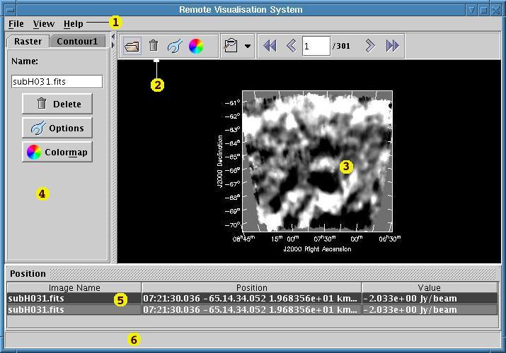
Figure 1: RVSViewer User InterfaceDisplay Canvas
As shown in Figure 1, Display Canvas is a panel where the images are drawn.
Image Detail Panel
The Image Detail Panel lists the images currently drawn on to the Display Canvas in a tabbed format. Each tab in the panel represents an image of type Raster or contour. The tab title is the image type. Each tab displays the name of the Raster image or Contour. The name by default is the file name of the image. However, the name field can be edited to change the name. Each tab also provides shortcut buttons to delete the image, modify image options and apply a different colormap to the image.
Position Information Panel
When the user clicks on the image the cursor position and the value are displayed in this panel.
Status Bar
Status Bar indicates the current status of the viewer. If the viewer is idle waiting for user input then the Status Bar is empty. However, if the viewer is currently communicating with the RVS server then an animation is displayed on the status bar to indicate this ( Figure 2).

Functions
View Remote Image
RVS can display any valid FITS image that can be accessed via a URL. To add an image to the canvas:
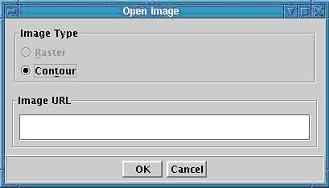
- Select Open Image from the File menu or click on the Open Image icon (
) or click Ctrl+O on the keyboard. The Open Image dialog box is displayed ( Figure 3). Select from Raster or Contour image type. Typically you would load an image as a raster and then overlay other images as contours. RVS is currently limited to viewing a single Raster image at a time. You are not permitted to overlay raster images. The Raster option will be disabled if a Raster image is already on display.
- Enter the image URL in the URL text box and press OK button.
A file is successfully loaded when you see the image drawn on the canvas and a new tab for the image appears in the Image Detail Panel. The time taken to load an image depends on:
- The size of the FITS file
- The bandwidth between your computer and the RVS Server
- The bandwidth between the RVS Server and the server where the image is located.
Delete Image
To remove an image from the canvas, select the tab corresponding to the image from the Image Detail Panel and click on the Delete button. When the image is successfully removed the image will no longer be displayed on the Display Canvas and the image details will be removed form the Image Detail Panel.
Clear Canvas/ Delete multiple images
To delete all images from the canvas:
- Press the Delete key on the keyboard or select Delete from the View menu or click on the Delete icon (
) .
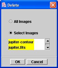
- The Delete dialog box shown in Figure 4 will pop up.
- Select All Images radio button to delete all images and press OK button.
- To remove more than one image click on Select Images radio button and select the required images from the list. Click OK. Selected images will be removed form the canvas.
Position Tracking
Click anywhere on top of an image to display the corresponding world or pixel coordinate in the Position Information panel. See section "Change Image Options" for options relating to position tracking. You can also double click in any cell of the position information table and press Ctrl+C on the keyboard to copy the position information and paste it into another application.
Zooming
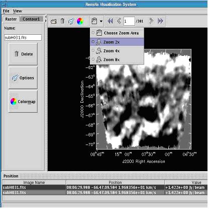
To zoom into an image you will have to first invoke the zoom mode. Press the Drop Down Icon (
) from the tool bar (Figure 5) and select from the four zoom options available.
The zoom icon on the toolbar changes to the selected zoom option. The icon will display depressed indicating that the viewer is now in zoom mode
. The zoom options are also available from View -> Zoom menu.
- Choose Zoom area (
) : This option zooms into a region. Click on the image and drag to draw a rectangle. This indicates the area that will be magnified. To zoom out hold the Ctrl key while drawing the rectangle.
- Zoom 2x (
): This option allows zoom in and out by a factor of 2. Click on the Display Canvas at the location where you want the magnification centered. Hold down the Ctrl key and click on the canvas to zoom out by a factor of two
- Zoom 4x (
) and Zoom 8x (
). These options are same as Zoon 2x except that zoon factor is 4 and 8 times respectively.
To exit the zoom mode and go back to normal mode just click on the Zoom icon. The icon will come back to normal position indicating that the viewer is in normal road. Clicking on the canvas now will no longer perform zoom operation.
Changing Color Map
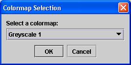
To apply a color map to the image select the Raster image tab from the Image Detail panel, or select Color Map from the View Menu or click on the Color map icon (
). The Colormap selection dialog will be displayed (Figure 6). Select from the list of predefined list and click OK. The Display Canvas will be updated accordingly.
Changing Channels in a Cube
When viewing a cube, users may step to different channels by using the Channel Change Control on the Tool Bar (Figure 7). This control provides the following options.
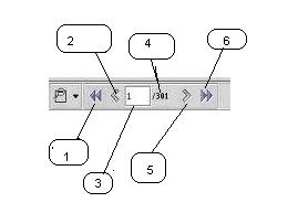
Figure 7: Channel Change Control
- First Channel (1): Displays channel 1.
- Back (2) : Displays channel one less than current channel number.
- Total channel count (4): total number of channels in the cube.
- Current Channel text box (3): This text box displays the current channel number. You can also type in a channel number that is less than total channel count and grater than 0 and press enter to directly go to that channel.
- Next (5): Display the channel one grater than the current channel.
- Last Channel (6) : Displays the last channel in the cube.
Change Image Options
You can change options of an image by clicking Options button on the image's corresponding tab in the Image Detail Panel. This will open a Image Options dialog (Figure 8) containing the options that you may alter. The list on the left side of the dialog lists the images currently displayed. You can also access the Image Options dialog through View -> Options menu and the Options tool bar icon (
).
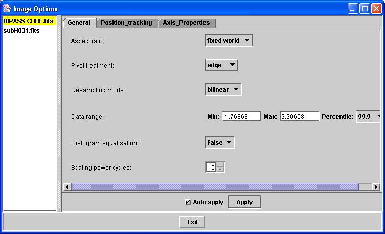
Figure 8: Image Options DialogAll options are categorised into different contexts and these are represented by one tab each. As shown in Figure 8 these categories are General, Position_Tracking and Axis_Properties. Axis_Properties is further divided into sub contexts: Hidden_Axis, Axis_Label_Propertis, Display_Axis and Axis_Labels (Figure 9). The contexts and their options are dependent on the type of image.
Figure 9: Image Options Dialog: Axis_PropertiesOptions available for all image types.
Display axes
In this tab, adjustments can be made to select how the data is sliced for display, i.e. which axes of the data are mapped to X and Y on the screen. The new selection will take effect immediately if Auto Apply is selected. Otherwise, the new selection will not take place until the Apply button at the bottom of the adjustment window is pressed. If you have selected the same axis for more than one display axis, then your request will be ignored, and you should correct your error, and press Apply again.
Hidden axes
This tab is only present when the image or array has more than three axes, and is used to set the location in the data along all of the axes which are not mapped to either X, Y or Z (movie) axes in the Display axes tab.
Position tracking
In this tab, adjustments can be made to how the coordinates under the pointer (mouse cursor, when clicked) are displayed.
By default, position tracking is enabled, so that when you click a mouse button with the pointer over an image, the data value and coordinate are shown in the image?s Position Display. You can turn position tracking off with the switch called Position Tracking at the bottom of the tab. Other options in this rollup are
- Position tracking - Absolute or relative
You may display absolute or relative (to the reference pixel) coordinates.
- Position tracking - World or pixel coordinates
You may display world or pixel coordinates.
- Position tracking - Fractional or integral pixel coordinates
A data lattice is discrete, but each pixel can be considered to extend over the range i?0.5. E.g. pixel [20, 30] in a 2D images covers the range [19.5, 29.5] to [20.5, 30.5]. By default pixel coordinates are presented integrally. If you like, this optional allows you to have them presented fractionally.
- Position tracking - Spectral unit
If the data contain a spectral axis, this menu will be included. It allows you to select the units for the presentation of the spectral coordinates (e.g. km/s or Hz etc). Conversion to km/s is only possible if the Spectral coordinate contains the rest frequency. In its absence, no conversion to km/s will be offered.
- Position tracking - Velocity type
If the data contain a spectral axis, this menu will be included. If you ask to see the spectral coordinate as a velocity, then this allows you to select the type of velocity definition (e.g. optical, radio etc.).
Axis labels
The parameters in this tab offer basic control over the axis labels (which by default are visible). You can toggle them on and off by selecting True/False for Axis labelling & annotation. The other parameters in this tab are pretty much self explanatory, and include text entries for the axis labels and control of whether tick marks or grid lines are drawn.
Axis label properties
In this tab, finer control over the axis label properties is provided.
Here you have control over whether the axis labels are shown as world coordinates or image pixel coordinates (1-relative). You may select whether the labels are relative (to the reference pixel) or absolute.
For Direction coordinates, you may select the units of the labels if they are relative. For Spectral coordinates you may select the units of the labels, and the velocity type. For other Coordinate types, you don't yet have further control over the units.
You can also choose the Direction coordinate reference type of the following J2000, B1950, GALACTIC, ECLIPTIC and SUPERGAL. Your coordinate grid will reflect these types.
You can also choose where to place your axis labels. The default Auto is usually sufficient, but other placements are available.
General
This tab has the parameters that most dramatically alter the generation of the raster map itself from the image or array data. The elements of this tab are:
- General - Aspect ratio
This option controls the dimensions with which data pixels are drawn to the screen. Fixed lattice means data pixels will be mapped to square pixels on the screen, in as much as the screen pixels themselves are square. Fixed world means that the aspect ratio of the pixels according to the coordinate system of the image will be honoured. Finally, selecting flexible will allow the raster map to stretch independently in each direction to fill as much of the canvas as possible.
- General - Pixel treatment
This option controls how individual data pixels are drawn to the screen. Selecting center means that pixels at the edge of the display will be drawn only from the centres inwards. That is, down the left hand border of the raster map, only the right-hand half of the pixels will be visible, and along the bottom of the raster map, only the upper half of the pixels will be visible. So for center, the raster map is drawn from the center of the bottom left pixel in the selected data to the center of the top right pixel in the selected data.
Selecting edge (the default) will change this behaviour such that all data pixels will be drawn fully on the screen. This would be useful for cases where only one of the display axes only has length one pixel.
- General - Resampling mode
This setting controls how the data are resampled to the resolution of the screen. Nearest refers to nearest neighbour resampling, where each pixel on the screen is colored according to the intensity of the nearest corresponding data pixel. The alternative, bilinear (default), applies a bilinear interpolation to produce smooth-looking images independent of the screen pixel dimensions of the data pixels. While bilinear resampling normally produces a better looking image, it can be significantly slower than nearest neighbour resampling, so be aware of this.
- General - Complex mode
If the data source (image or array) is Complex, then this menu allows you to select whether you wish to see the magnitude, phase, real or imaginary part.
Raster Options
These options are available for Raster images only.
General - Histogram equalisation
The default value for this option is False. When enabled for raster maps, some internal optimisation of colors from the colormap (or color channel) is made. The number of colors allocated to a given range of data is proportional to the fraction of pixels whose pixel intensities lie in that range. Thus color cells are allocated where they are needed most.
General - Scaling power cycles
This option offers further control over the mapping of data values to color cells from the colormap. The overall process in selecting a color for a particular pixel is as follows: the data value of the pixel is clipped lie between the data minimum and maximum as specified elsewhere in this General tab. Then, according to this option which is described below, this clipped pixel intensity is mapped to an index between 0 and the number of colors available in the selected colormap. The color which is in the colormap at this position, which itself is controlled by the current stretch, shift, contrast, brightness and invert settings of the colormap, is then drawn for this particular pixel.
So, the scaling power cycles option controls the mapping of clipped pixel intensities to color look-up values. When this is set to zero, a straight line connects (domainMin, rangeMin) and (domainMax, rangeMax) on a plot where the domain is the input data values constrained to the range given by the data min and max sliders, and the range runs from 1 to number of colors in the selected colormap
As the scaling power decreases from zero, the curve deviates from the straight line, rising above it, such that an increasing fraction of the available colormap is used for data values close to the data minimum. This curve is calculated using a log function.
As the scaling power increases from zero, the curve deviates from this straight line, falling below it, such that an increasing fraction of the available colormap is used for data values closer to the maximum. The curve is calculated using an exponential function.
Contour Options
The following options are available for contour images only.
General - Contour scale factor
The contour levels given will be multiplied by the factor entered in this option before being drawn.
General - Level type
This option indicates whether the vector of contour levels, specified in the Contour levels box, multiplied by the scale factor, are absolute levels (that is, in the native units of the image), or are instead fractional levels, where 0 is mapped to the lowest pixel intensity in the image, and 1 is mapped to the highest.
General - Line width
This option controls the thickness of the contour lines.
General - Dash negative contours?
Set this option to True if you would like contours of negative values in your data to be dashed rather than solid lines.