S o u t h e r n G a l a c t i c P l a n e S u r v e y
SGPS Data Server User Manual
Contents
IntroductionField descriptions
Sample queries
Getting FITS
Going to the movies
Viewing channel maps
Introduction
This is the user manual for the SGPS Data Server system. The readership for this documentation should be for typical users of the system; primarily astronomers. The manual will progress through the entire process from input, to getting the FITS results, through to viewing the result as an animation or channel map sample.
Explanation of fields
Longitude is the abscissa along the x-axis or horizontal axis for the image cubes. The units are determined by the pull-down menu to the right of this text field. This will be the horizontal centre for the face of the cube. The units can be in gl/gb, B1950 ra/dec and J2000 ra/dec.Latitude is the y-ordinate along the y-axis or vertical axis for the image cubes. The units are determined by the pull-down menu to the right of this text field. This will be the vertical centre for the face of the cube. The units can be in gl/gb, B1950 ra/dec and J2000 ra/dec. The typical range within the cubes on latitude is from -1.5 degrees to 1.5 degrees.
Sub-region width is the horizontal width of the region. The centre of this width will be the abscissa specified in the "Longitude" field. For example, if the "Longitude" field was "287" and the sub-region width was "10", then the horizontal range of the sub-region's face is 282-292 (5 degrees each way of 287).
Units are in degrees.
Sub-region height is the vertical height of the region. The centre of this height will be the y-ordinate specified in the "Latitude" field. For example, if the "Latitude" field was "0" and the sub-region width was "1", then the vertical range of the sub-region's face is -0.5 to 0.5 (0.5 degrees each way of 0).
Units are in degrees.
Velocity range defines the depth of the cube along the z-axis. The units are in km/s.
Note: If there is no velocity value for either the minimum or maximum values, then they are assigned the minimum and maximum value of the original cube. e.g. if original cube has velocity range of -171 to 200 and user inputs:
- no min velocity and no max velocity, then the min and max velocities are assigned to -171 and 200 respectively.
- min velocity = 0 and no max velocity, then min = 0 and max = 200.
- no min velocity and max = 100, then min = -171 and max = 100.
Colour scheme tells the server the colour of the mask that should be placed over the image. The default is "Heat" as it is Naomi's favourite. If you experience difficulty with seeing colours, it may be advisable to use the "Grey" option.
Survey tells the server which survey they want to obtain the data from. For example, it could be from Parkes+ATCA or just Parkes.
Sample queries
Following are a number of screen shots of sample queries. There are two example queries here:- A query using galactic coordinates, "Heat" colour mask
- A query using J2000 ra/dec coordinates "Grey" colour mask
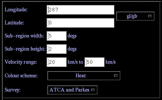 |
| Figure 1: Query using galactic coordinates. Note that the pull down bar next to the "Longitude" and "Latitude" text fields is set to "gl/gb". Also note that the values for "Longitude" and "Latitude" are decimal values because they are in units of degrees. |
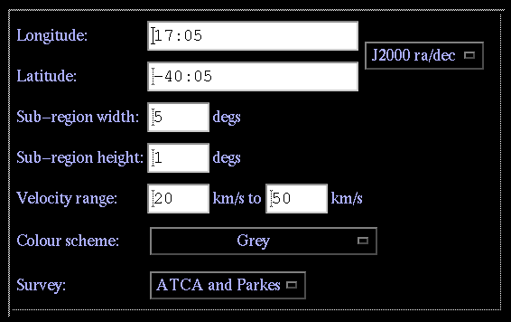 |
| Figure 2: Query using J2000 ra/dec coordinates. Note that the pull down bar next to the "Longitude" and "Latitude" text fields is set to "J2000 ra/dec". Also note that the values for "Longitude" and "Latitude" are written in the form of hours:minutes:seconds and degrees:minutes:seconds because they are in units of Right Ascension and Declination. |
Getting FITS
The following screen shots show the resulting page after clicking on the "Submit" button on the initial page.If results are present (if not, a message will appear indicating this) a table of results will be visible, as illustrated in Figures 3 and 4.
The first set of rows shows some statistics of the original larger cube.
The second set of rows shows some statistics of the smaller sub-cube.
The third set of rows shows three different methods of accessing or viewing the results. To get the FITS file, you will need to right-click on the link in the first box and save the file on your local computer and then view it with the appropriate software (e.g. kvis). Left-clicking on this will generate a lot of garbage as the browser is not capable of decoding the file. Links to two facilities for viewing the sub-cube are provided in the next two boxes. This is particularly useful for those users who do not have the appropriate software to view the FITS file with. The two viewing facilities provided are:
- A movie, indicated by the "play button".
- A channel map, indicated by a sample channel map.
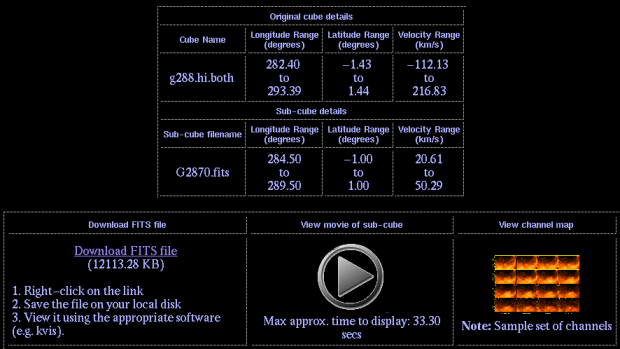 |
| Figure 3: The resulting page after clicking on "Submit" from Figure 1. |
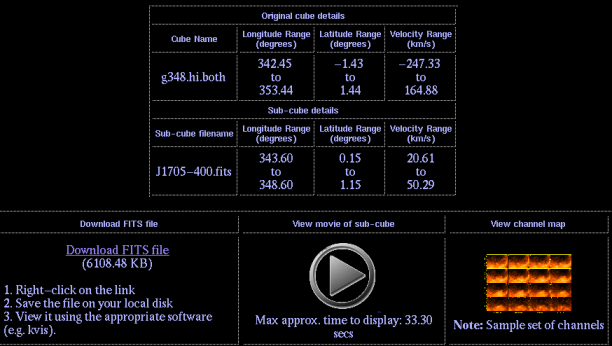 |
| Figure 4: The resulting page after clicking on "Submit" from Figure 2. |
Going to the movies
Viewing a movie of the cube is one of the most effective ways of looking at your results. However, this can be a slow process, especially if you query with a large velocity range. As you can see from Figures 3 and 4, along with the movie is an estimate of the time it will take to display it. This estimate has a direct relationship with the number of planes in the cube.It is important to note that if you have made a previous query with the same longitude and latitude values but changed other fields, you may still get the same image after clicking this. This is due to the web-browser caching the image and you will need to press Shift+Refresh to reload the image.
Another thing to note is that the first round of frames (e.g. if the velocity range is 20-50, then it is the first 30 frames from 20-50) displayed will be quite slow. This is because the browser is still downloading each frame. But once the first iteration is over, the browser makes use of the cached images and the animation will be much smoother and faster.
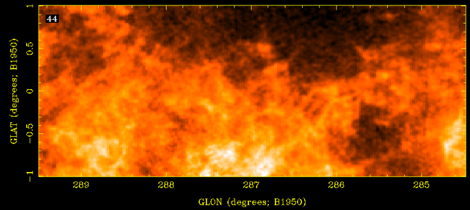 |
| Figure 5: A still shot of the movie generated after clicking on the "play button" in Figure 3. |
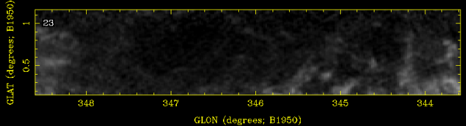 |
| Figure 6: A still shot of the movie generated after clicking on the "play button" in Figure 4. |
Viewing channel maps
Channel maps graph out each channel as a sequence of the images along the z-axis of the cube, from the first plane to the end.Due to the large images and potential for numerous maps needed for large velocity ranges, the SGPS Data Server limits the number of channels displayed to 16. Hence, if there are more than 16 channels in the sub-cube, a sample of the channels will be displayed.
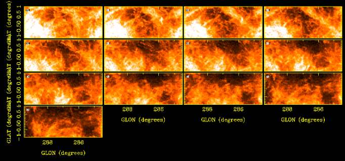 |
| Figure 7: The resultant channel map after clicking on the channel map link in Figure 3. |
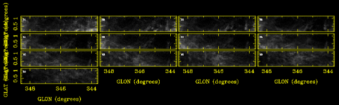 |
| Figure 8: The resultant channel map after clicking on the channel map link in Figure 4. |