MNRF Upgrade: 12-mm System on the ATCA
[The System | Performance | Notes for Observers | Science ]
Project Personnel
Project Leader: Graham Moorey, ATNF
Receiver Group
Project Scientist: Ravi
Subrahmanyan
The System
All six antennas of the Compact Array are now equipped with 12 mm receivers covering the frequency range 16-26 GHz. The receiver package contains a compact corrugated feed horn with octave bandwidth followed by cryogenically cooled orthomode transducers and low-noise front-end amplifiers, and a local oscillator and conversion system that translates selected 12-mm frequencies to 6 & 3 cm bands. The low-noise amplifiers are InP integrated circuits (MMICs) using HEMT devices, designed in-house by the ATNF receiver group. The receiver package, before being enclosed in the cryogenic dewar, is shown in the left panel, on the right is shown the receiver on the rotating turret at the vertex of a Compact array antenna. The 12mm system shares a common dewar with the 3mm receivers, the separate feed horns at the top of the dewar are moved to the Cassegrain focus of the Compact Array antennas using the rotator positioning system. Because the 12 and 3 mm receivers have separate feed horns, observations cannot be simultaneous in the 12 and 3 mm bands. The high-frequency local oscillator for the first down-conversion of the 12-mm frequencies to 3/6-cm bands is derived in each antenna from a 11.2-15.6 GHz reference that is synthesized at the central site and sent out on an optical carrier via single-mode fibres to all the antennas.
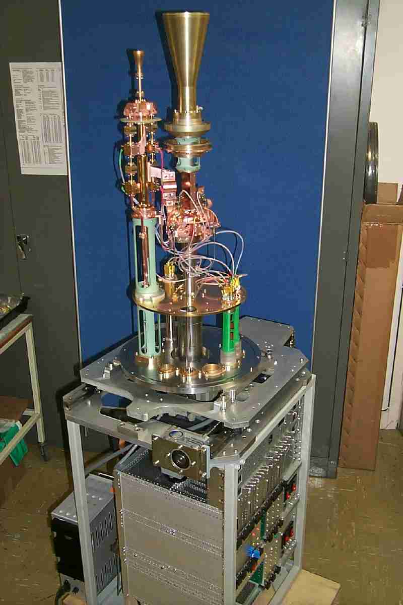

(Click on images for larger versions)
Permitted observing frequencies/bandwidths
The Compact array allows simultaneous observing in two polarisations at each of two frequencies. For 12-mm observations, the centres of the two observing bands must both be in the range 16 to 26 GHz; additionally, the two frequencies are required to be at most 2.7 GHz apart and have integer MHz values. Either or both frequencies can have bandwidths of 64 or 128 MHz. The first frequency can have a narrow bandwidth of 4, 8, 16 or 32 MHz. See the list of available correlator configurations in the Compact array users guide to find one that suits your astronomy. The Compact Array does not carry out online Doppler corrections.
Field of view
The FWHM of the antenna primary beam is 2.75 arcmin at 18 GHz. At any other frequency in the 12 mm band, the FWHM is given by {2.7485 - 0.1077(f-18)} arcmin, where f is the frequency in GHz.
Polarization
Dual linear. The system provides IFs that correspond to orthogonal linear polarizations. The X and Y polarizations correspond to E-fields at P.A. 45 and -45 degrees with respect to the vertical.
System Performance
The first figure below shows measurements of the system temperature referred to the face of the feed horn: the contributions from receiver noise plus dish and ground spillover, atmospheric brightness in good weather conditions, and 3 K sky are shown separately. The second figure shows measurements of the antenna gain with the optics focussed for the middle of the 12 mm band. The third figure shows the sensitivity in Jansky assuming a correlator efficiency of 88%.
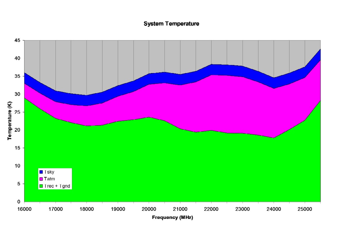

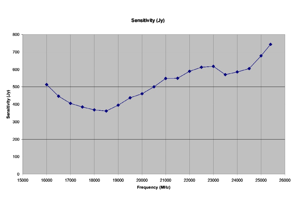
(Click on images for larger versions)
The sensitivity of the array for Fourier synthesis imaging may be estimated using the ATCA sensitivity calculator .
The high frequency local oscillator has a phase noise less than 6 degrees R.M.S. and, consequently, the amplitude decorrelation in the 12 mm band because of local oscillator phase jitter is less than 1 per cent.
Notes for Observers
Continuum observers who wish to image sources using the 12-mm system with best sensitivity and a 2 x 128 MHz bandwidth may choose to place their band centres at frequencies 128 MHz apart and close to 18.5 GHz. Recommended frequencies are 18496 and 18624 MHz. The coupling of the calibration noise into the feed horns has problems at frequencies above 25.4 GHz; therefore, system temperature calibration may have large errors at these frequencies and this top end of the band ought to be used with extreme caution, preferably avoided.
At present, observations in all bands and frequencies are made with a single fixed focus setting: observers do not change the antenna focus.
A guide to processing 12-mm data in MIRIAD is available.
Antenna pointing issues
The Global pointing solutions that are determined after every reconfiguration are invoked when the option POINTING:GLOBAL is selected in SCHED. In this mode, the antenna pointing errors are measured to have an R.M.S. value of about 6 arcsec; pointing errors as much as 20 arcsec might be expected in specific antennas.
If better antenna pointing is desired, reference pointing is recommended. Assuming that all six antennas are available for the observation and all four IFs are being used, CAOBS requires to be primed for the reference pointing with commands "SET POINT_ANTENNAS 123456" and "SET POINT_IFFLAG 1234" and "SET POINT_PATTERN 2" at the start of the observing. The reference pointing is implemented in two separate steps: (i) pointing solutions are determined as part of the observing strategy, using SCTYPE:POINT & POINTING:REFPNT scan on an unresolved calibrator located close to the source on the sky, and (ii) these solutions are used for the pointing model using POINTING:OFFSET option while observing the secondary calibrator and source. The reference pointing solutions should be recomputed every 1-2 hours or whenever the antennas move significantly in azimuth/elevation or whenever the ambient temperature or weather conditions change significantly. The pointing solutions ought to be determined on a reasonably strong calibrator, say 0.5 Jy at the minimum. The reference solutions computed from the last point scan and the offsets currently being applied are displayed in the CAMON page /point. With reference pointing, the R.M.S. pointing error is measured to be within 2 arcsec.
Primary calibration of the flux scale
The flux density of 1934-638 does appear constant at 12mm, at least over 6 months, and a model of its spectrum has been built into MIRIAD's calibration software; therefore, an observation of 1934-638 may serve as the primary flux density calibrator. See the note on measurements of the flux density of 1934-638 at 12 mm by Bob Sault. Alternately, observers might choose to include an observation of a planet. The planet should have sufficient flux density ( exceeding 0.5 Jy) at least on some baselines and should ideally be observed within the elevation range in which the observations of the secondary calibrator are made. The planetary ephemerides can be found at the JPL planetary website. SCHED recognises major planets, the Sun and Moon, and automatically computes appropriate ephemeris; see the Compact array users guide for details. MIRIAD has two tasks which assist in using planets to calibrate data: (i) PLPLT, which plots visibility amplitudes for a given planet at a given time and frequency as a function of baseline, and (ii) PLBOOT, which calibrates a source in a data set containing at least one observation of a planet.
Secondary calibrators
The calibrators database gives information on potential sources that may be used to measure the interferometer amplitude/phase calibration. A round-trip phase correction machinery automatically corrects for the changes in electronics path length in real time; therefore, the astronomical secondary calibration observations are for taking out the atmospheric path changes and any errors in the baseline parameter determinations. The on-line system temperature calibration takes out the temporal changes in the electronics gain but does not correct for atmospheric opacity; therefore, the secondary calibrator amplitudes are important for correcting for the elevation dependent changes in the opacity.
Bandpass calibration
Spectral-line observers are advised to observe bandpass calibrators with every observing session/day and separately correct each days data for the bandpass complex gain before merging datasets.
SCHED related issues
Observers at 12 mm are advised to disable the averaging option, i.e., set AVERAGING=1. This is because the changes in the differential atmospheric phase between the antennas might very well cause a decorrelation in visibility amplitudes over long integration times. Additionally, users of SCHED are warned against using GLOBAL command to set frequencies because this circumvents the checks in SCHED that guard against the use of "illegal" frequencies.
If changing frequencies during an observing session
Changes in the observing frequency usually cause a change in the frequency of the first local oscillator. The synthesizer is located in the central site and the phase of this reference frequency in a round trip to each antenna and back is used to estimate the instrumental phase which is used on-line as a round-trip phase correction. The consequence of this system for observers is that the recorded phase could have arbitrary jumps whenever the observing frequency changes. Therefore, observers who wish to switch between frequencies during their observing sessions are advised to commence and end observations at each frequency with a record of the visibilities on the secondary calibrator.
Coarse attenuators
The total power changes significantly with elevation, with weather conditions and across the 16-25 MHz band. Usually, the observing software automatically switches in/out phaseless (fine) attenuators and maintains optimal power levels at the samplers. However, operator intervention becomes necessary if a coarse attenuation step should be required (ASSISTANCE would alert the observer to the condition that the power levels are outside the range in which the sampler levels can operate). Coarse attenuation steps may be invoked using the CAOBS command "SET COARSE CA0n XXXX", where n is the antenna number and XXXX is the attenuation required. The coarse attenuations take values 0-3 and the four values correspond to the four IF chains A1, B1, A2 & B2 in that order. However, the coarse attenuators are not phase-less! Therefore, observers are advised to record visibilities on the phase (secondary) calibrator before and immediately after any change in coarse attenuators, and break (GPBREAK) gain solutions at the times when coarse attenuators were altered.
Atmosphere related issues
The atmospheric contribution is dependent on frequency, elevation angle and the water vapour column, which might be estimated given the ambient temperature, pressure and humidity (see the /weather page in CAMON for these parameters). There is a MIRIAD task OPPLT which estimates the sky brightness temperature (3K CMB sky as seen through the atmosphere plus the atmospheric contribution) and opacity for clear skies. MIRIAD's ATLOD has an option that corrects 12 mm visibility amplitudes for atmospheric opacity based on weather data that is recorded in the RPFITS data files.
Science
The first 12 mm fringes on all six antennas were obtained on April 16, 2003. Some examples of science with the 12 mm system that have made it to the ATNF newsletter are listed below.